Surrogate Model Explorations

Explorations lets you systematically explore and optimize design spaces using trained surrogate models. Instead of running inference on one design at a time, you build multi-physics systems on a visual canvas, sweep across hundreds of parameter combinations, and run optimization algorithms to find optimal designs, all without writing code.

A 128-point Design of Experiments (DOE) sweep completes in seconds. A 420-evaluation multi-objective optimization completes in ~16 minutes. The equivalent traditional simulations would take weeks to months.

Highlights

• Guided workflow: Start exploration → Build system → Configure variables → Choose sweep or optimize → Review results
• Visual system builder: Wire together Input, Geometry, Model, Script, and Output blocks on a canvas
• Multi-physics optimization: Combine surrogate models from different physics disciplines (e.g., CFD and FEA) in a single study
• Design space sweeps: Run DOE sweeps to map how outputs respond to input changes
• Multi-objective optimization: Find Pareto-optimal designs that balance competing objectives using NSGA-II or weighted optimization
• Rich visualizations: Pareto front, response driver maps, and geometry galleries showing the physical shapes the optimizer discovered
• Fast iteration: Export results to CSV, duplicate runs, and refine your exploration

Prerequisites

Before you begin:

• AI Physics must be enabled for your organization
• One or more trained surrogate models — Train models using the guidance in Training Surrogate Models, or use available example models
• A parametric geometry (optional, for geometry optimization) — Upload a Python geometry generator, or use a static mesh if only scalar parameters vary
• Familiarity with single-point inference — Understanding how a single surrogate prediction works will help you understand what sweeps and optimization do at scale

Key Concepts

Explorations

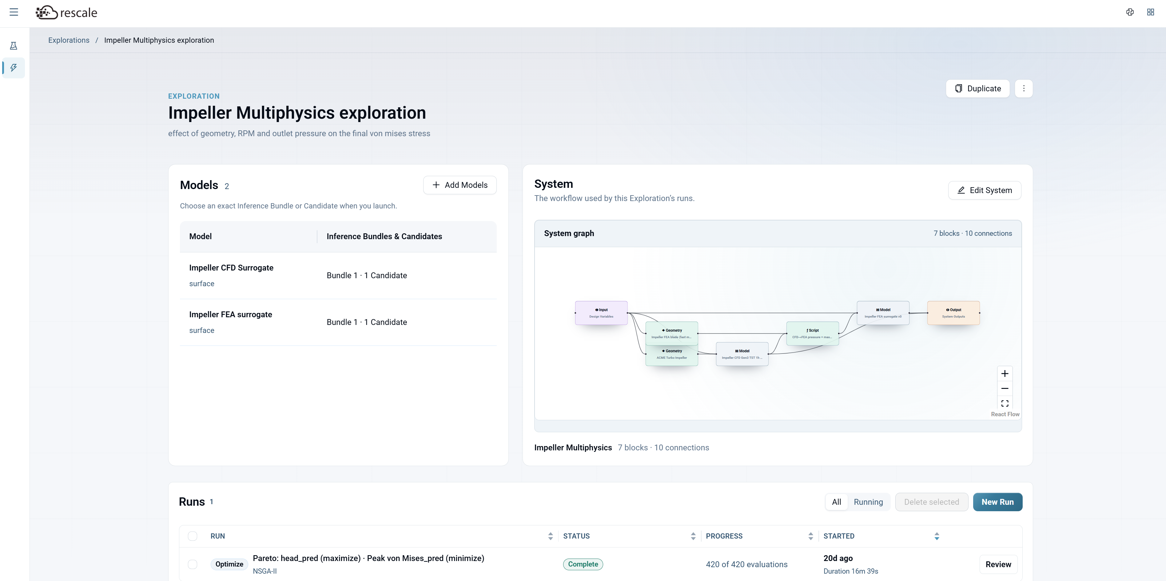
An Exploration groups together the models, system definition, and runs for a design study. Each Exploration has:

• Models — The surrogate models used in this study, with their Inference Bundles and Candidates
• System — A visual graph defining how data flows from inputs through geometry, models, and scripts to outputs
• Runs — Sweep or optimization runs executed against the system, each with its own results

You manage Explorations from the Explorations page (accessible from the left sidebar), where you can search, create, and launch runs.

System Builder

The System Builder is a visual canvas where you design multi-physics pipelines by connecting blocks. It is the core of Explorations: this is where you define what your study computes for each design variant.

Available block types:

Category	Block	Role	Example
Inputs and Outputs	Input	Design variables that change across sweep/optimization	D0, d0, RPM, AngleBeta1, etc.
Inputs and Outputs	Output	Collected results from the system	head_pred, Peak von Mises, etc.
Physics	Geometry	Parametric geometry generator that creates a mesh from parameters	Impeller FEA blade, ACME Turbo Impeller
Physics	Model	Trained surrogate model that predicts outputs	Impeller CFD Gen3, Impeller FEA surrogate v0
Logic	Script	Custom Python logic to bridge data between models or compute derived quantities	CFD→FEA pressure + masks
Logic	Math	Mathematical operations on scalar values	Unit conversions, derived variables
Logic	Constraint	Bounds or feasibility conditions on variables or outputs	Stress limits, geometric constraints

Data flows left to right across the canvas. You drag blocks from the left panel, drop them on the canvas, and connect their ports. The system validates connections automatically.

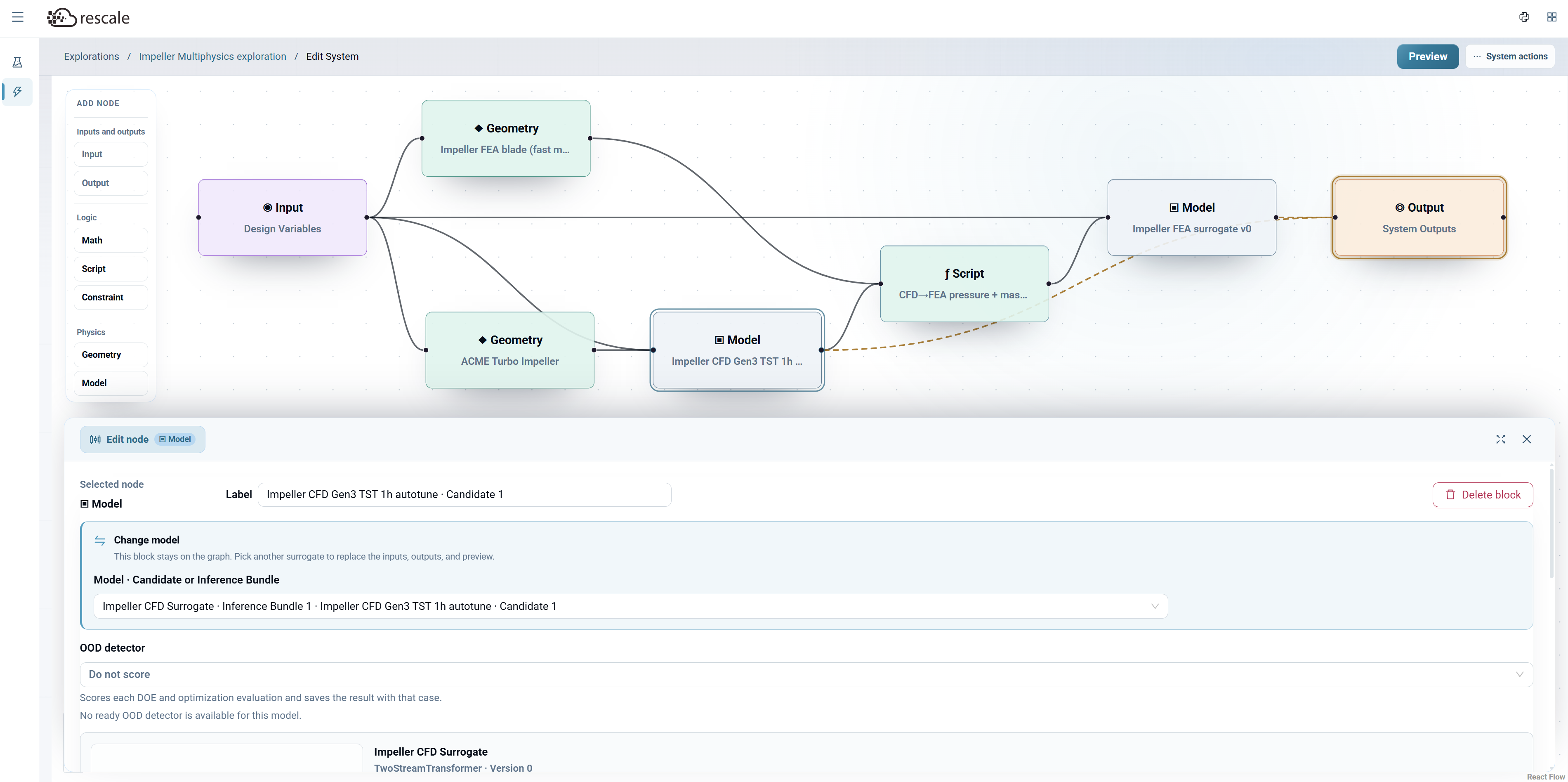
Multi-physics example: An impeller optimization might connect Input → two Geometry blocks (FEA blade mesh + turbo impeller mesh) → a CFD Model + an FEA Model → a Script node (to map CFD outputs as FEA boundary conditions) → Output.

Sweep (DOE)

A sweep evaluates a set of design points sampled from the input parameter space. It maps how outputs respond to changes in inputs, giving you a broad picture of the design space before committing to optimization.

Sampling strategies:

• Latin Hypercube — Space-filling sample that covers the design space efficiently. Recommended for high-dimensional problems (many parameters).
• Full Factorial — Evaluates every combination of parameter levels. Thorough but grows exponentially (5 levels x 7 parameters = 78,125 combinations).
• One-at-a-time — Varies one parameter at a time while holding others constant. Useful for understanding individual parameter effects.
• Random sample — Randomly samples points from the design space. Simple but less efficient coverage than Latin Hypercube.

Optimization

Optimization uses algorithms to intelligently search for the best designs. It evaluates designs, learns which regions of the parameter space are promising, and concentrates its search there.

Single Objective vs Multi-Objective

Choose between two optimization types:

• Single Objective — Searches for the design that optimizes one score. Best when you have a clear single metric to optimize (e.g., minimize drag, maximize efficiency). You can combine multiple outputs into a single objective using an expression (e.g., Cl / Cd or Cd * Cd).

• Multi-Objective — Keeps competing goals on a Pareto front. Best when you have conflicting objectives (e.g., maximize head while minimizing stress). The optimizer finds designs where you cannot improve one objective without worsening another.

Single Objective Configuration

For Single Objective optimization:

1. Objective Output: Select the output variable to optimize from your system.
2. Direction: Choose Minimize or Maximize.
3. Combine Outputs By: Select Expression to define a custom objective function combining multiple outputs (e.g., Cl / Cd for lift-to-drag ratio).

Multi-Objective Configuration

For Multi-Objective optimization:

1. Add each objective using the Quick Add Output buttons or manually specify outputs.
2. For each objective:
   • Direction: Choose Maximize or Minimize
   • Search Weight: Set the relative importance (default 1.0 for equal weighting)
3. Click + Add Objective to add more objectives.

Downweight unfamiliar designs (optional checkbox): When enabled, the optimizer prioritizes designs closer to the training data distribution, reducing the risk of trusting predictions in unexplored regions of the design space.

Multi-Objective Methods

Choose between two multi-objective optimization approaches:

Weighted Search Combines objectives into one direction-aware weighted score, then the selected optimizer searches that score. Every objective is still retained for Pareto analysis. Best for problems where you have a clear preference weighting between objectives.

NSGA-II Non-dominated Sorting Genetic Algorithm II. Evolutionary algorithm that maintains Pareto diversity by evolving a population over generations. Best for exploring the full Pareto front when you don't know the ideal trade-off in advance.

Weighted Search Optimizer

When using Weighted Search, select an optimizer strategy:

Global, Hybrid, or Local:

• Global — Population search across the full parameter space. Best for broad nonconvex spaces and loose initial guesses.
• Hybrid — A rough global sweep followed by deterministic polish. Balances exploration and refinement.
• Local — Gradient-based methods that converge quickly from a good starting design.

Optimizer Method (varies by strategy):

For Global:

• Differential evolution — Population search across the full box. Best for broad nonconvex spaces and loose initial guesses.
• Bayesian optimization — Builds a surrogate of the objective and samples intelligently. Best for expensive objectives or noisy data.
• CMA-ES — Covariance Matrix Adaptation Evolution Strategy. Adaptive evolutionary algorithm good for continuous optimization.
• Random search — Samples randomly across the parameter space. Baseline method.

For Hybrid:

• DE → L-BFGS-B — Differential evolution followed by L-BFGS-B. Best for a rough global sweep followed by deterministic polish.
• DE → BFGS — Differential evolution followed by BFGS.
• DE → SQP — Differential evolution followed by Sequential Quadratic Programming.
• CMA-ES → L-BFGS-B — CMA-ES followed by L-BFGS-B.
• CMA-ES → BFGS — CMA-ES followed by BFGS.
• CMA-ES → SQP — CMA-ES followed by Sequential Quadratic Programming.

For Local:

• L-BFGS-B — Limited-memory BFGS with bounds. Fast gradient-based method for smooth response surfaces with a good starting design.
• BFGS — Broyden-Fletcher-Goldfarb-Shanno. Quasi-Newton method for unconstrained optimization.
• SQP (SLSQP) — Sequential Least Squares Programming. Gradient-based method that handles constraints.

Parameters:

• Max Full Iterations: Maximum number of optimization iterations (default: 20)
• Max Parallel Evals: Number of evaluations to run in parallel (default: 1)

NSGA-II Parameters

When using NSGA-II for multi-objective optimization:

Parameter	Default	Description
Population size	20	Number of designs evaluated per generation
Generations	20	Number of evolutionary cycles
Crossover probability	0.99	Likelihood of combining two parent designs
Mutation probability	0.00	0 = uses 1/variable_count (adaptive)
Random seed	0	Set for reproducibility

Total evaluations = population_size + (generations x population_size) = 20 + (20 x 20) = 420

Run Artifacts

After configuring the search method (Sweep or Optimize), you can specify which artifacts to generate during the run. This controls what data and visualizations are saved for each evaluated design.

Generate configured assets for the best design (checkbox): When enabled, the system automatically generates geometry files and visualization assets for the best design found during optimization.

Capture PNG Previews: Control when geometry preview images are generated:

• Best improvements — Captures a new Geometry PNG whenever the best design improves (recommended for optimization runs)
• All cases — Captures PNG previews for every evaluated case (useful for sweeps where you want to review all geometries)
• None — Skips PNG generation to save storage and processing time

Preview-Capable Blocks: For each Geometry and Model block in your system, configure:

• MESH DATA (.vtm): Check to export the full mesh data file for external visualization or post-processing
• PNG PREVIEW (.png): Check to generate a rendered preview image
• COLOR BY: Select which field to visualize on the surface (e.g., Surface, Pressure, Temperature)

Run Label: Provide a descriptive name for this run (e.g., "Impeller Multiphysics"). This label appears in the exploration's run history and helps you distinguish between multiple optimization attempts.

The Artifact Status area displays real-time progress as artifacts are generated (e.g., "Generating best-improvement assets from ACME Turbo Impeller, Impeller FEA blade").

Pareto Front

When you have multiple objectives (e.g., maximize head_pred AND minimize Peak von Mises), the Pareto front shows the set of "non-dominated" designs, meaning designs where you cannot improve one objective without worsening another.

• Points ON the Pareto front are all equally optimal
• Points NOT on the front are suboptimal (a better design exists somewhere)
• Choosing between Pareto-optimal designs is an engineering judgment, not a math problem

Create an Exploration

Navigate to the Explorations tab in AI Physics Training or AI Physics Inference. If you don't have any explorations yet, you'll see an empty page with a prompt to start.

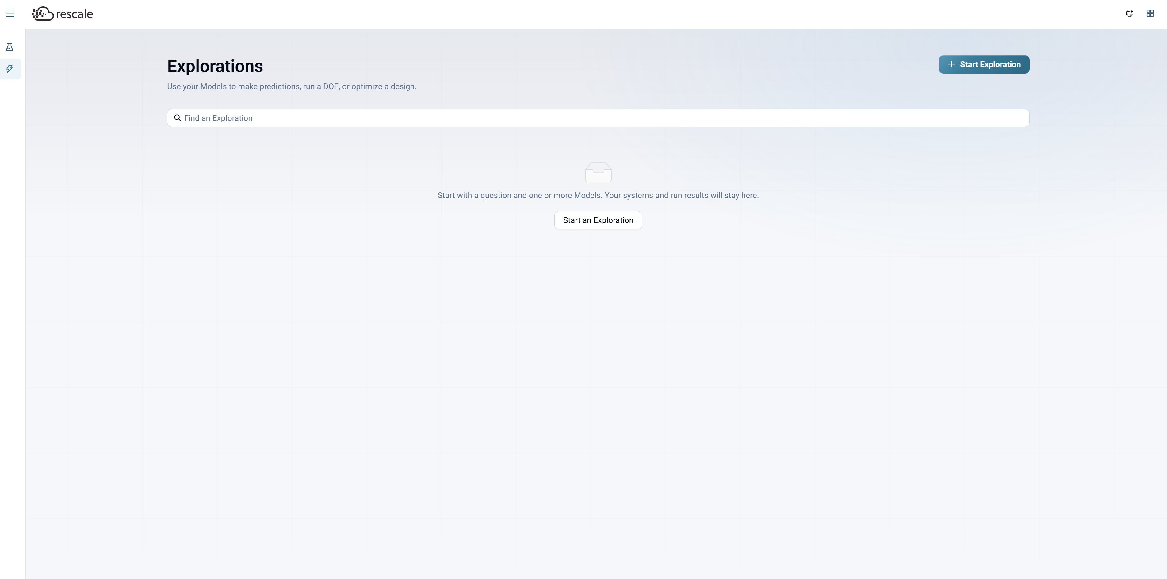
Click + Start Exploration to begin.

Provide Exploration Details

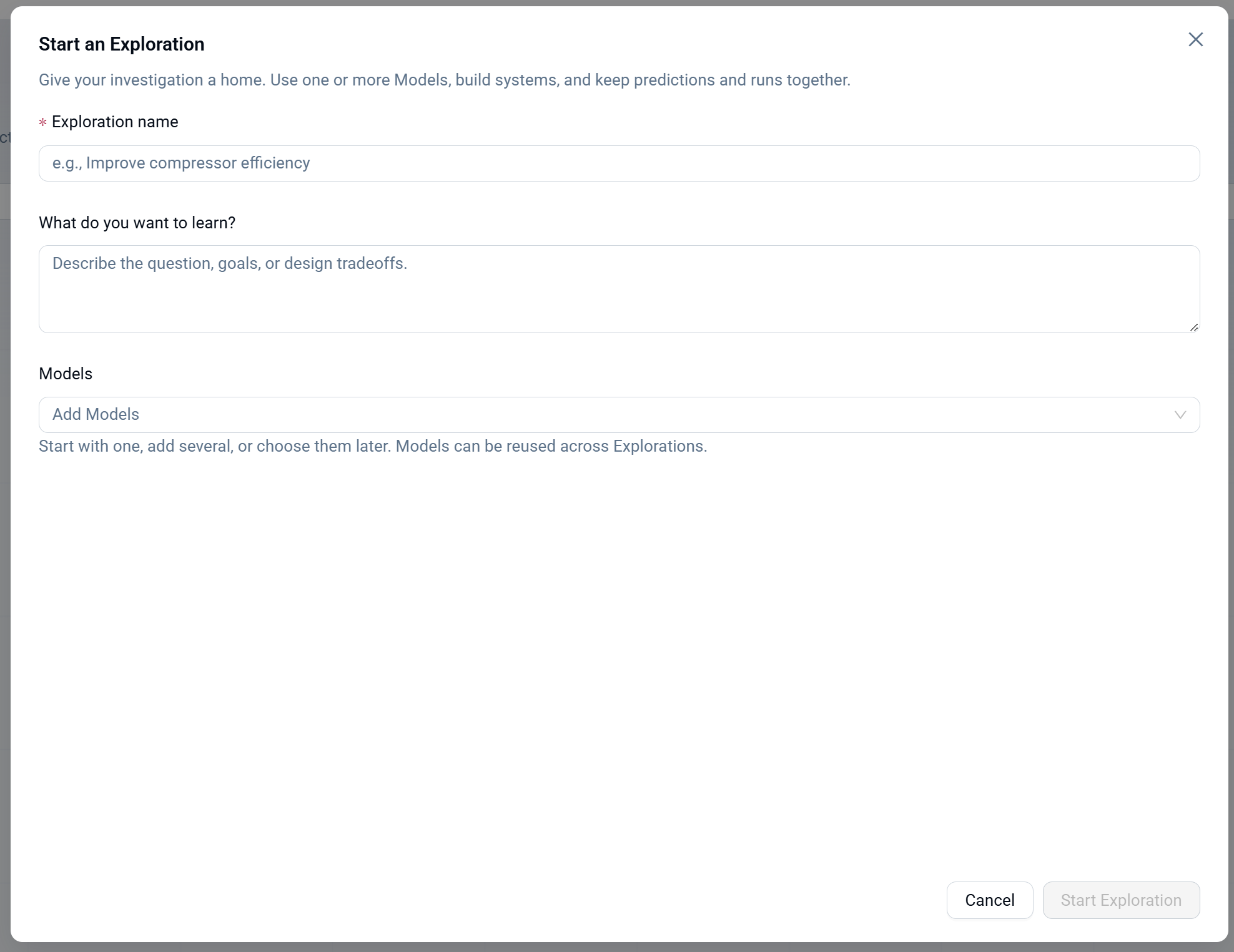
In the Start an Exploration dialog:

1. Enter an Exploration name (e.g., "Improve compressor efficiency").
2. Describe What do you want to learn? Give the question, goals, or design tradeoffs you're investigating (e.g., "Optimize AoA to minimize drag").
3. Click Add Models and select the trained surrogate models you want to use in this study. You can add one model or several for multi-physics studies.
4. Click Start Exploration.

You're taken to the exploration home page, which shows three sections: Models, System, and Runs.

Build the System

From your exploration home page, click + Build System to define how inputs flow through geometry, models, and logic to produce outputs.

Add Blocks to the Canvas

The System Builder opens with a visual canvas and a left panel listing available block types:

• Inputs and outputs: Input, Output
• Logic: Math, Script, Constraint
• Physics: Geometry, Model

Drag blocks onto the canvas and connect them by drawing wires between ports. Data flows left to right.

Add Geometry

If your exploration involves parametric geometry, add a Geometry block:

1. Drag a Geometry block from the left panel onto the canvas.
2. Click the Geometry block to configure it.
3. In the Parametric definition section, choose your geometry generator (e.g., "ACME Turbo Impeller").
4. Optionally select a Remesh target points value if you want to control mesh resolution.

Once configured, the Geometry block shows:

• Inputs: The design variables (parameters) the geometry depends on (e.g., D0, d0, b2, AngleBeta1, AngleBeta2).
• Geometry preview: A 3D preview of the generated mesh with parameter details.
• Connections: How the geometry connects to other blocks (Design Variables → Geometry).

Configure Surrogate Models

Add Model blocks for each surrogate model in your exploration:

1. Drag a Model block onto the canvas.
2. Click the Model block to configure it.
3. The panel shows:
   • Model name and version (e.g., "Impeller CFD Surrogate · Inference Bundle 1 · Candidate 1")
   • Inputs: Where the model gets its inputs from (e.g., Design Variables, Geometry)
   • Outputs: The predicted fields and scalars the model produces

For multi-physics systems, add multiple Model blocks and use Script blocks to bridge data between them (e.g., mapping CFD pressure outputs to FEA boundary conditions).

Set Inputs and Outputs

Add an Input block at the start of your system to define design variables, and an Output block at the end to collect results.

• The Input block exposes the design variables you'll sweep or optimize (e.g., D0, d0, RPM, AngleBeta1).
• The Output block collects the outputs you want to track (e.g., head_pred, Peak von Mises stress).

Connect all blocks in a logical flow: Input → Geometry → Model → Output (or more complex chains for multi-physics).

Preview the System

Click Preview (upper right) to verify your system works before creating runs.

The Preview panel shows:

• Graph Readiness: Whether the system is ready to run.
• Inputs: Number of input design variables.
• Outputs: Number of output variables.
• Mesh outputs: Number of geometry outputs.
• System components: List of all blocks (INPUT, GEOMETRY, MODEL, SCRIPT, OUTPUT) with details.
• Geometry block previews: 3D renders of generated geometries.

If the system preview shows "Ready", you can proceed to create runs. If there are issues, the preview will flag them.

Create a New Run

Once your system is built and previewed, return to the exploration home page and click New Run to start a sweep or optimization.

The run workflow has three steps: Configure, Explore, and Execute.

Step 1: Configure

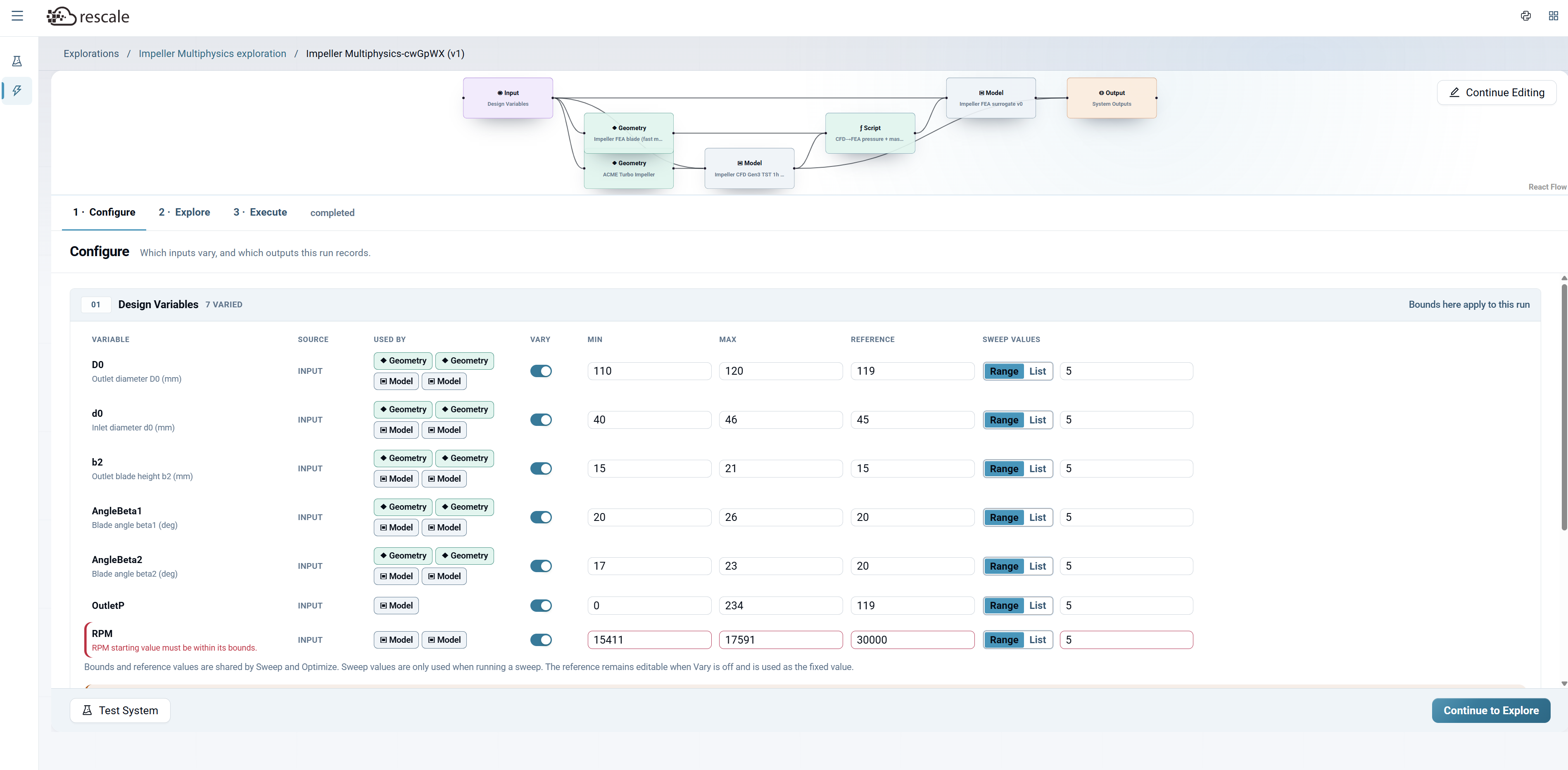
The Configure step shows your system graph at the top and configuration options below.

Design Variables

Lists all variables discovered from your Input block. For each variable:

• Variable: Name and description (e.g., "D0 - Outlet diameter (D0 mm)")
• Source: Where the variable comes from (INPUT)
• Used By: Which blocks consume this variable (e.g., Geometry, Model)
• Vary: Toggle ON to include in the sweep/optimization, OFF to hold at the reference value
• Min / Max: Bounds for the search space
• Reference: Default or center value
• Sweep Values: Choose Range (evenly spaced) or List (specific values), and specify count

Toggle Vary ON for the variables you want to explore, and set their Min/Max bounds.

Output Variables

Output variables are automatically included based on your system's Output block. These are the results you'll analyze after the run completes.

Click Continue to Explore when configuration is complete.

Step 2: Explore

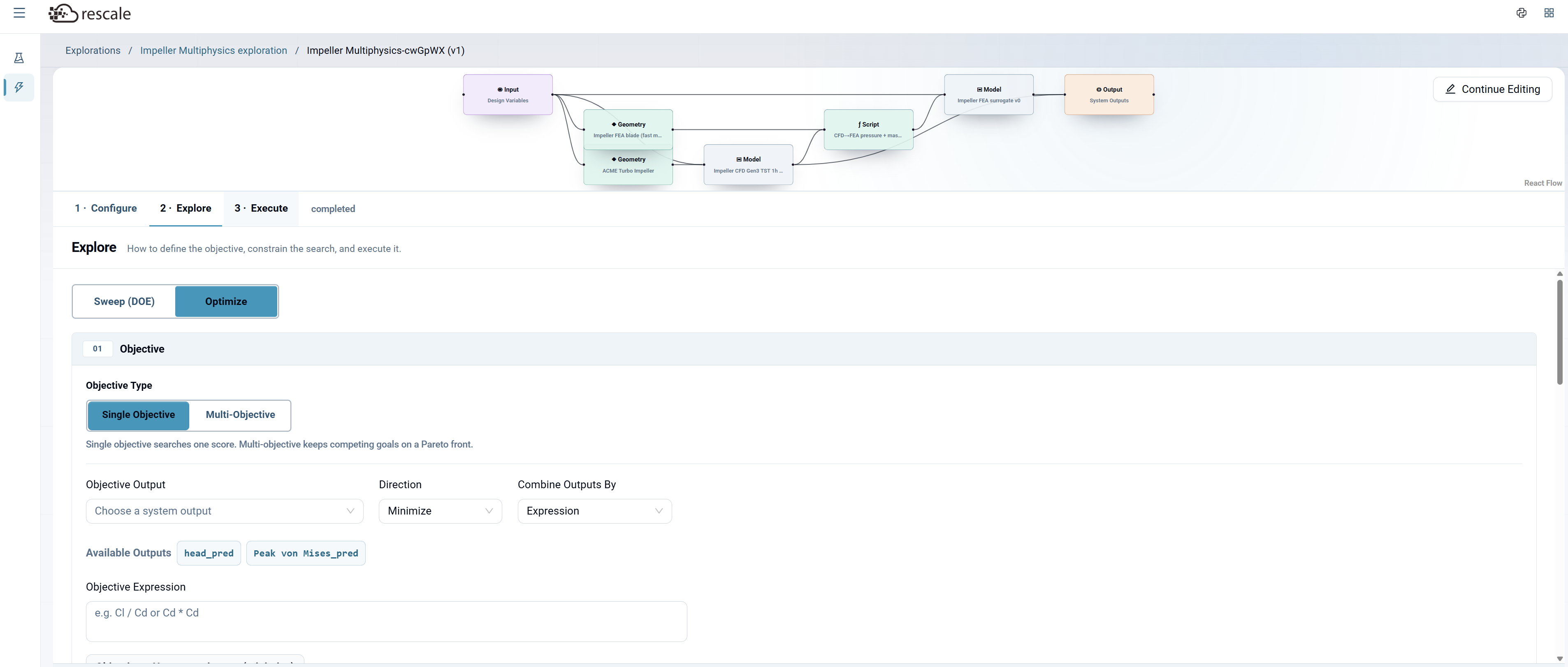
Choose how to explore the design space: Sweep (DOE) or Optimize.

Sweep (DOE)

Configure sweep parameters:

• Sampling strategy: Choose Latin Hypercube, Full Factorial, One-at-a-time, or Random sample (see Sweep (DOE) in Key Concepts for guidance)
• Sample count: How many design points to evaluate (e.g., 64, 128, 200)
• Max cases: Upper bound on evaluations
• Execution plan: Choose Auto (recommended), Serial, or Manual

Click Run Sweep to start.

Optimize

Choose Objective Type: Select Single Objective or Multi-Objective (see Single Objective vs Multi-Objective in Key Concepts for guidance).

Configure Objectives:

For Single Objective:

1. Select the output variable to optimize
2. Choose Minimize or Maximize
3. Optionally define a custom expression combining multiple outputs (e.g., Cl / Cd)

For Multi-Objective:

1. Add objectives using Quick Add Output buttons
2. Set Direction (Maximize/Minimize) and Search Weight for each
3. Click + Add Objective to add more

Optionally check Downweight unfamiliar designs to prioritize designs closer to the training data.

Choose Search Method (Multi-Objective only):

Select Weighted Search or NSGA-II. For method details, parameters, and guidance on which to choose, see Multi-Objective Methods in Key Concepts.

For Weighted Search: Choose optimizer strategy (Global/Hybrid/Local) and method, then configure iterations and parallel evaluations.

For NSGA-II: Configure population size, generations, crossover/mutation probabilities, and seed.

Configure Run Artifacts (optional): Choose which artifacts to generate (mesh data, PNG previews, best-design assets). See Run Artifacts in Key Concepts for details.

Run Label: Provide a descriptive name for this run.

Click Run Optimization to start.

Step 3: Execute

After the run completes, the Execute step displays results.

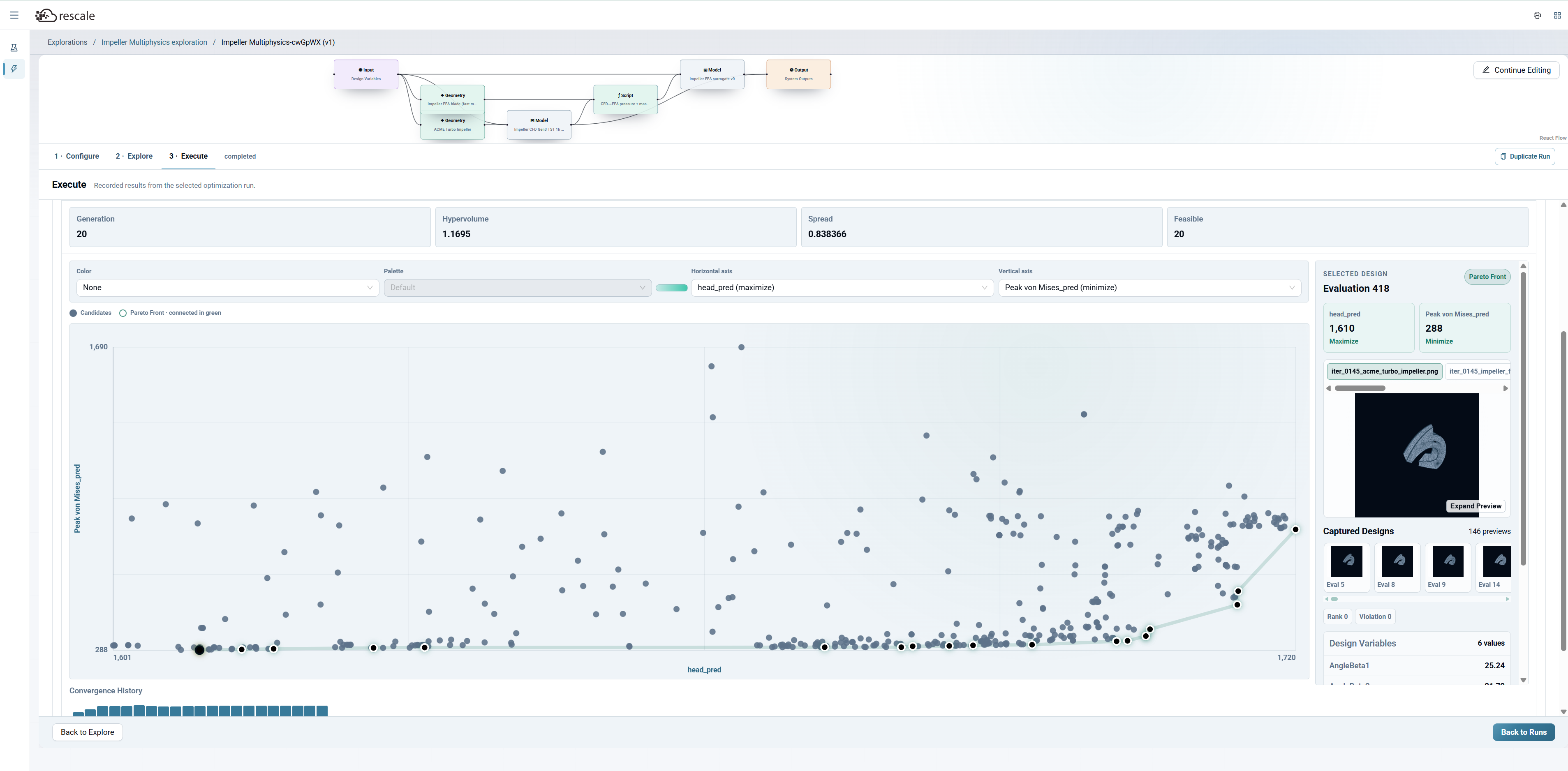
Overview: Pareto Front

For multi-objective optimization, the results show a Pareto front: the set of designs where you cannot improve one objective without worsening another.

• Each point represents one evaluated design.
• Points on the Pareto front (highlighted or clustered at the edge) are optimal.
• Points not on the front are suboptimal.

The visualization includes:

• 2D scatter plot: X-axis and Y-axis map to your objectives (e.g., head_pred vs Peak von Mises_pred).
• Captured Designs: Thumbnail gallery showing geometry previews for selected designs (e.g., Eval 5, Eval 8, Eval 9, Eval 14).
• Design Variables: Values for each design variable in the selected design.

Response Driver Map

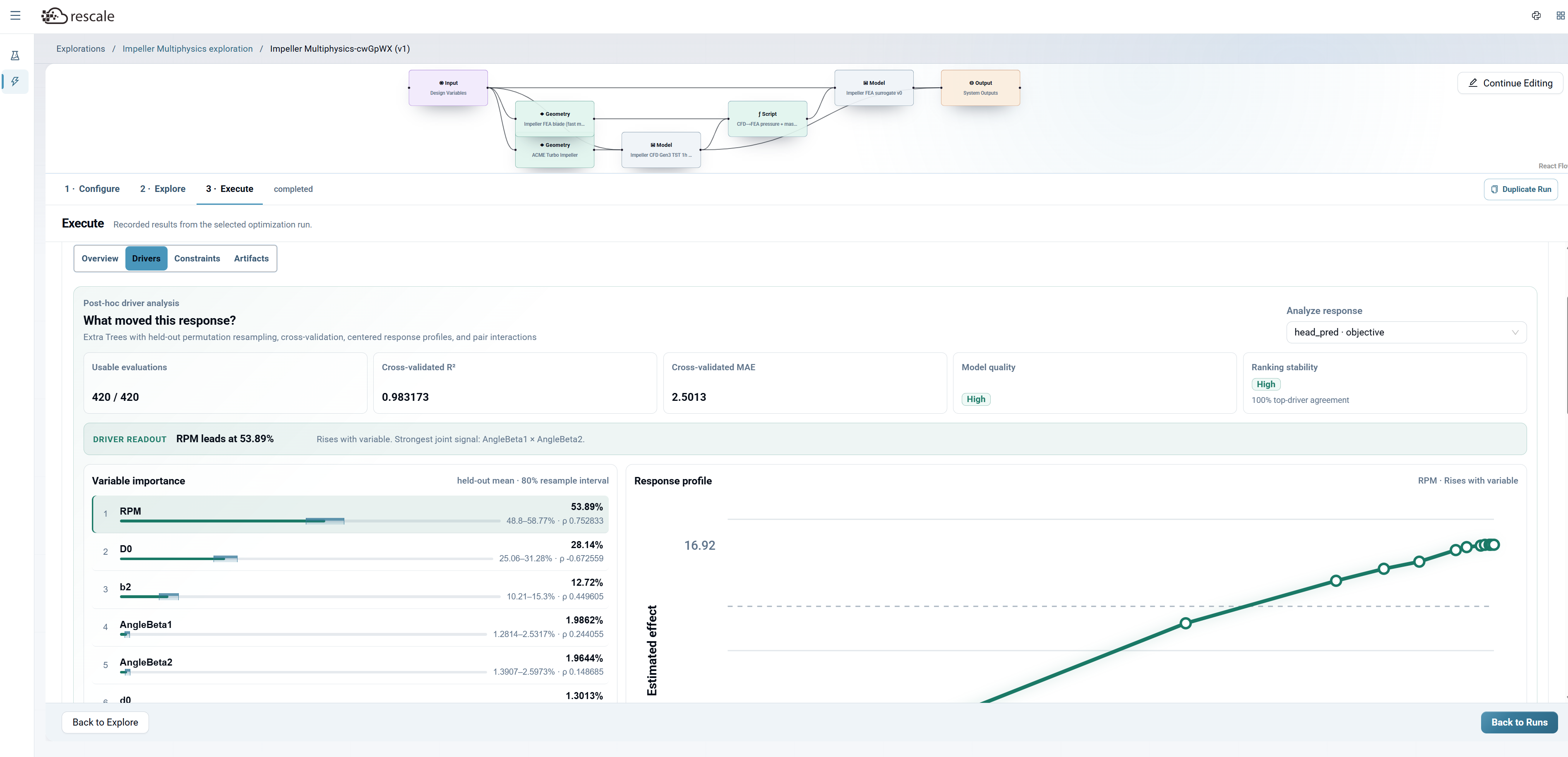
The Drivers tab shows sensitivity analysis, naming which input parameters most influence each output.

The Response driver map displays a grid:

• Rows: Design variables (e.g., D0, RPM, d0, AngleBeta1, b2, AngleBeta2)
• Columns: Output variables (e.g., head_pred, Peak von Mises_pred)
• Cell values: Percentage importance and direction indicator (arrows)

Higher percentages mean the input variable has a stronger influence on the output.

Artifacts

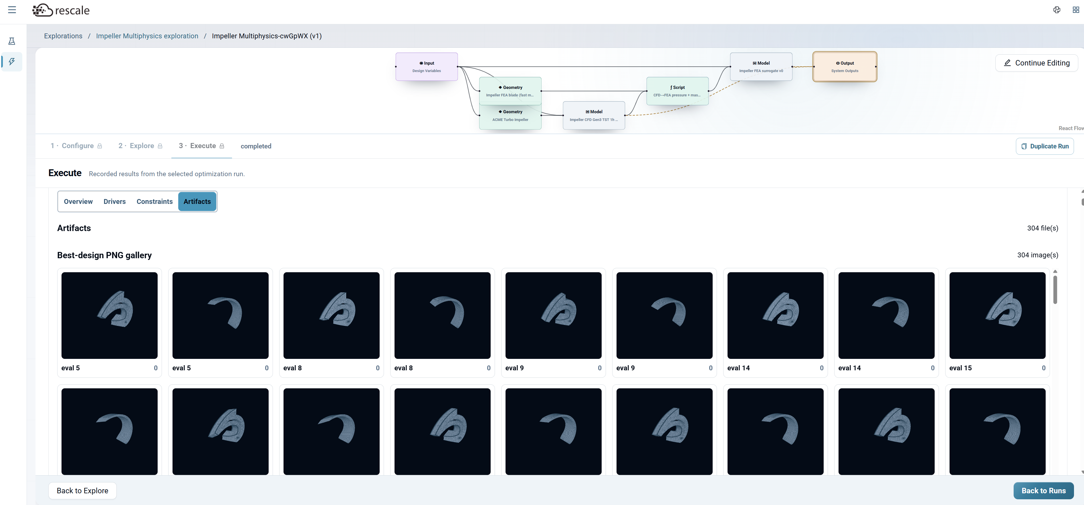
The Artifacts tab displays generated files from the run, including:

• Geometry gallery: Rendered images of the geometries explored during the optimization or sweep. Each thumbnail shows the physical shape for one evaluation (e.g., eval 252, eval 254, eval 257).

This lets you visually compare the shapes the optimizer discovered, not just the numbers.

Export and Iterate

• Export CSV: Download all case data for offline analysis.
• Duplicate Run: Create a copy of this run to iterate with different settings.
• Back to Runs: Return to the exploration home page to create new runs or review past results.

Common Workflows

Workflow A: Exploration-First (Recommended for new users)

1. Start Exploration: Provide name, description, add models
2. Build System: Add Input → Geometry → Model → Output blocks, configure each
3. Preview: Verify system works
4. New Run: Configure design variables (set Min/Max, toggle Vary ON)
5. Explore: Choose Sweep (DOE) with 128–200 points
6. Execute: Review results, understand design space
7. New Run: Configure same variables, choose Optimize with multi-objective
8. Execute: Review Pareto front, response drivers, geometry gallery
9. Export: Download optimal designs

Workflow B: Direct Optimization (When objectives are known)

1. Start Exploration: Add models
2. Build System: Configure blocks
3. Preview: Verify
4. New Run: Configure variables, choose Optimize directly
5. Explore: Set objectives (Maximize/Minimize), configure NSGA-II
6. Execute: Review Pareto front
7. Export: Download optimal designs

Workflow C: Multi-Physics Optimization

1. Start Exploration: Add CFD + FEA Models
2. Build System: Input → Geometry (CFD mesh) + Geometry (FEA mesh) → CFD Model → Script (bridge CFD→FEA) → FEA Model → Output
3. Preview: Verify data flows correctly between models
4. New Run: Configure design variables affecting both physics
5. Explore: Optimize with competing objectives (e.g., maximize head, minimize stress)
6. Execute: Review Pareto front balancing multi-physics trade-offs, inspect geometry gallery
7. Export: Download best multi-physics designs

Workflow D: Parameter-Only (No geometry variation)

1. Start Exploration: Add Model
2. Build System: Input → Model → Output (no Geometry block)
3. Preview: Verify system with scalar inputs only (pressure, RPM, angles)
4. New Run: Configure scalar variables
5. Explore: Sweep or Optimize
6. Execute: Results show output sensitivity to scalar parameters (no geometry gallery)

FAQ

How many design points should I use for a sweep? 64–200 for initial exploration. Latin Hypercube with 128 samples gives good coverage for up to ~10 parameters. Increase if you need finer resolution in specific regions.

Should I sweep first or go straight to optimization? Sweep first if you're unfamiliar with the design space. The results help you understand the objective landscape and set meaningful optimization targets. Skip the sweep if you already know your objectives from prior analysis.

How long does optimization take? Depends on population size, generations, and system complexity. With default settings (20 population × 20 generations = 420 evaluations), expect ~16 minutes for a multi-physics system with geometry. Simpler parameter-only systems are faster.

Can I stop a sweep or optimization early? Yes. You can stop at any time. Partial results are preserved and can be reviewed.

Can I combine CFD and FEA models in one study? Yes, this is a core capability. When you start an exploration, add both models. In the System Builder, wire them together: Input → Geometry blocks → CFD Model → Script (to map CFD outputs as FEA boundary conditions) → FEA Model → Output.

What does the Preview button do? Preview validates your system before you create runs. It checks that the graph is connected correctly, shows how many inputs and outputs you have, and generates geometry previews so you can verify the system works.

What does the Artifacts tab show? The Artifacts tab displays generated files from the run, including a geometry gallery, holding rendered images of the geometries explored during the sweep or optimization. Each thumbnail shows one evaluated design. This lets you visually compare the physical shapes the optimizer discovered, not just the numbers.

What does the Response Driver Map show? The Response Driver Map (in the Drivers tab) shows sensitivity analysis, naming which input parameters most influence each output. Higher percentages mean the input variable has a stronger effect on the output. Use this to understand what drives your objectives.

How do I use this with models that have no geometry input (scalar-only)? Build your system without a Geometry block: Input → Model → Output. The system works with scalar inputs only (e.g., pressure, RPM, angles). All sweep and optimization features work the same way. The Artifacts tab won't show a geometry gallery since there's no geometry.

What's the difference between Single Objective and Multi-Objective optimization? Single Objective finds the design that optimizes one metric (e.g., maximize head_pred). Multi-Objective finds a Pareto front of designs that balance multiple competing objectives (e.g., maximize head_pred AND minimize stress). Choose Multi-Objective when you have trade-offs.

When should I use Weighted Search vs NSGA-II for multi-objective optimization? Use Weighted Search when you have a clear preference weighting between objectives (e.g., "efficiency is twice as important as cost"). The weighted objective becomes a single score that fast gradient-based optimizers can exploit. Use NSGA-II when you want to explore the full Pareto front without committing to weights up front. It maintains diversity across trade-offs and helps you understand the full range of optimal designs.

Which optimizer should I choose for Weighted Search? Start with Global (Differential evolution) if you're exploring a new design space with no good starting point. Use Hybrid (e.g., DE → L-BFGS-B) for the best balance of exploration and refinement, because it does a rough global sweep then polishes with a gradient method. Use Local (e.g., L-BFGS-B) only when you have a good initial design and a smooth objective surface, as it converges quickly but can get stuck in local optima.

What sampling strategy should I use for sweeps? Latin Hypercube is recommended for most cases, because it provides efficient space-filling coverage for high-dimensional problems. Use Full Factorial when you have few parameters (2-3) and want to see every combination. Use One-at-a-time when you want to isolate individual parameter effects. Random sample is a baseline method but less efficient than Latin Hypercube.

Glossary

Term	Definition
Exploration	A workspace grouping models, a system definition, and runs for a design study
System	A visual graph of connected blocks defining how inputs flow through geometry, models, and logic to produce outputs
System Builder	The visual canvas editor for creating and editing systems
Inference Bundle	A trained model version packaged for inference
Candidate	A specific checkpoint or variant within an Inference Bundle
DOE	Design of Experiments — systematic method for sampling a parameter space
Latin Hypercube	Sampling strategy that ensures each parameter range is evenly covered
Full Factorial	Sampling strategy that evaluates every combination of parameter levels
One-at-a-time	Sampling strategy that varies one parameter at a time while holding others constant
Random sample	Sampling strategy that randomly samples points from the design space
Single Objective	Optimization that searches for the design optimizing one metric or expression
Multi-Objective	Optimization that finds designs balancing multiple competing objectives on a Pareto front
Weighted Search	Multi-objective method that combines objectives into one weighted score for optimization
NSGA-II	Non-dominated Sorting Genetic Algorithm II — evolutionary multi-objective optimizer
Global optimizer	Population-based search across the full parameter space (e.g., Differential evolution, CMA-ES)
Hybrid optimizer	Two-phase optimization combining global exploration with local refinement (e.g., DE → L-BFGS-B)
Local optimizer	Gradient-based method that converges quickly from a good starting design (e.g., L-BFGS-B, BFGS, SQP)
Pareto front	Set of designs where no design is better on ALL objectives simultaneously
Non-dominated	A design that cannot be improved on one objective without worsening another
Parametric geometry	A geometry defined by parameters — change parameters, change the shape
Trade space	The space of all possible output combinations for a given input domain