Training Surrogate Models

In AI Physics Training, you create a model by selecting your simulation data, configuring inputs and outputs, reviewing data quality, and launching a training run. The model learns the relationship between your simulation inputs and outputs. AI Physics offers two training methods: Auto Tune (recommended) for automated hyperparameter optimization, and Manual for full control over every training parameter.

Highlights

• Unified model creation flow: Select simulation jobs, validate cases, configure inputs/outputs, and launch training—all in one streamlined workflow
• Analytics and insights: Review outliers, examine test/training split coverage, and see recommendations for filling design space gaps before training
• Auto Tune (Recommended): Automatically explores multiple hyperparameter configurations in parallel, drops weak candidates, and keeps the best model — work that would take weeks of manual experimentation
• Four production-ready architectures: DoMINO, GeoTransolver, MeshGraphNet (built on PhysicsNeMo 2.0 and licensed under Apache 2.0 and PyTorch) and TwoStreamTransformer (Rescale developed)
• Built-in evaluation dashboards: R² scores, residual distributions, and 3D error visualizations to validate model quality

Prerequisites

Before you begin:

• AI Physics Training must be open: Launch a Training Session from Model Builder in the Rescale platform, then open AI Physics Training. See Launching a Training Session if you haven't set up a session yet.
• Simulation data must be ready: Your Rescale jobs should have completed successfully with Metadata Extraction and AI Extraction Automations enabled. See Launching a Training Session for details on preparing simulation data.

Create a New Model

When you open AI Physics Training for the first time, the Models page is empty. Click + New Model to begin.

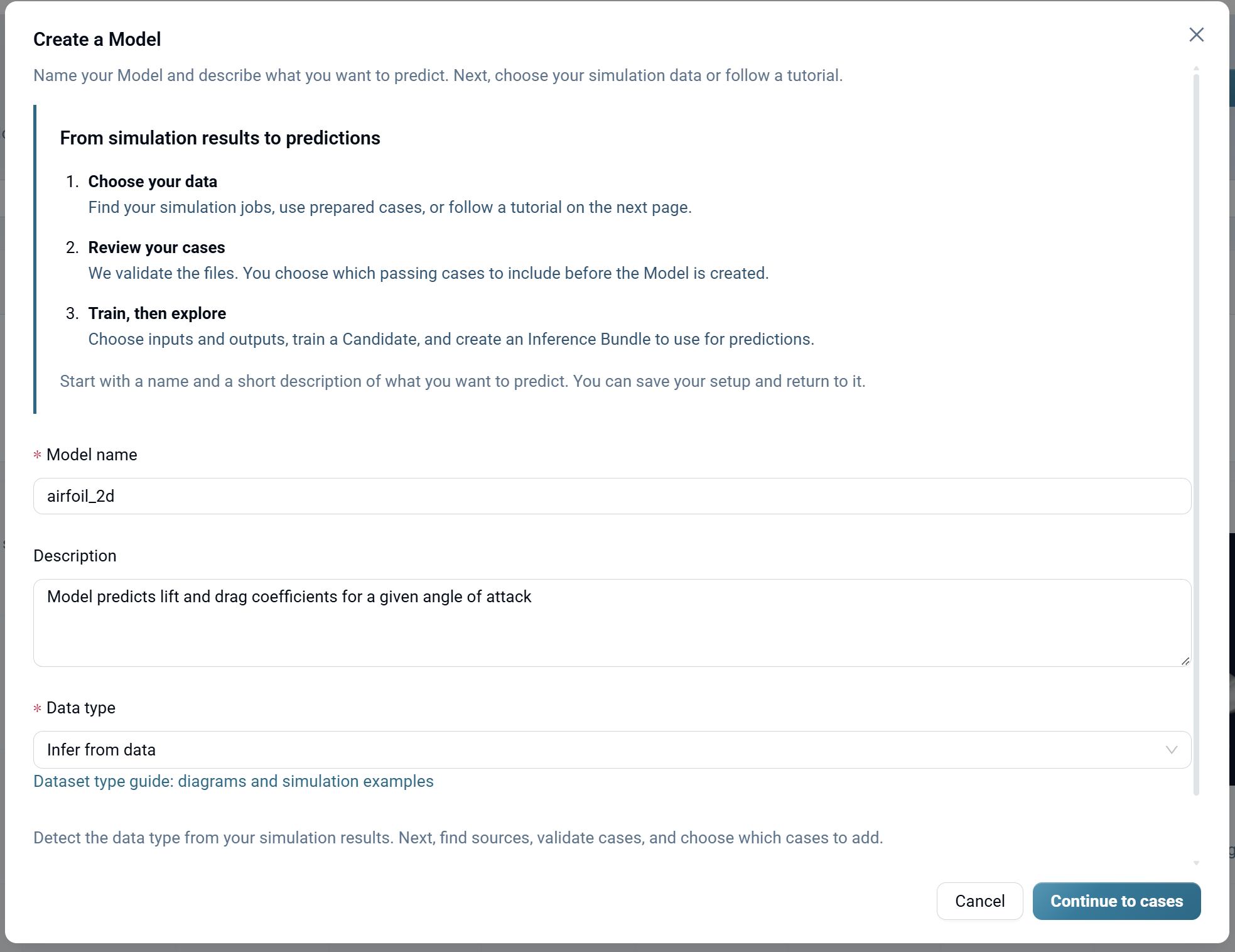
Provide Model Details

1. Enter a Model name (e.g., "airfoil_2d").
2. Optionally, add a Description explaining what the model predicts (e.g., "Model predicts lift and drag coefficients for a given angle of attack").
3. Select a Data type:
   • Surface: For surface-based predictions (e.g., pressure distribution on an airfoil surface).
   • Volumetric: For volumetric field predictions (e.g., velocity or temperature fields).
   • FEA Static: For static structural analysis predictions (e.g., stress, strain, displacement on static loads).
   • FEA Deformation: For deformation and dynamic structural analysis predictions (e.g., large deformation, crash, impact).
   • Forming simulation: For metal forming and manufacturing process predictions (e.g., sheet metal forming, stamping).
   • Point cloud: For point cloud-based predictions where data is represented as discrete points rather than a mesh.
   • Infer from data: AI Physics automatically detects the data type from your simulation results (recommended when unsure which type to choose).
4. Click Continue to cases.

Select and Validate Cases

Cases are individual simulation runs that the model learns from. Each case represents one set of input parameters and its corresponding simulation output.

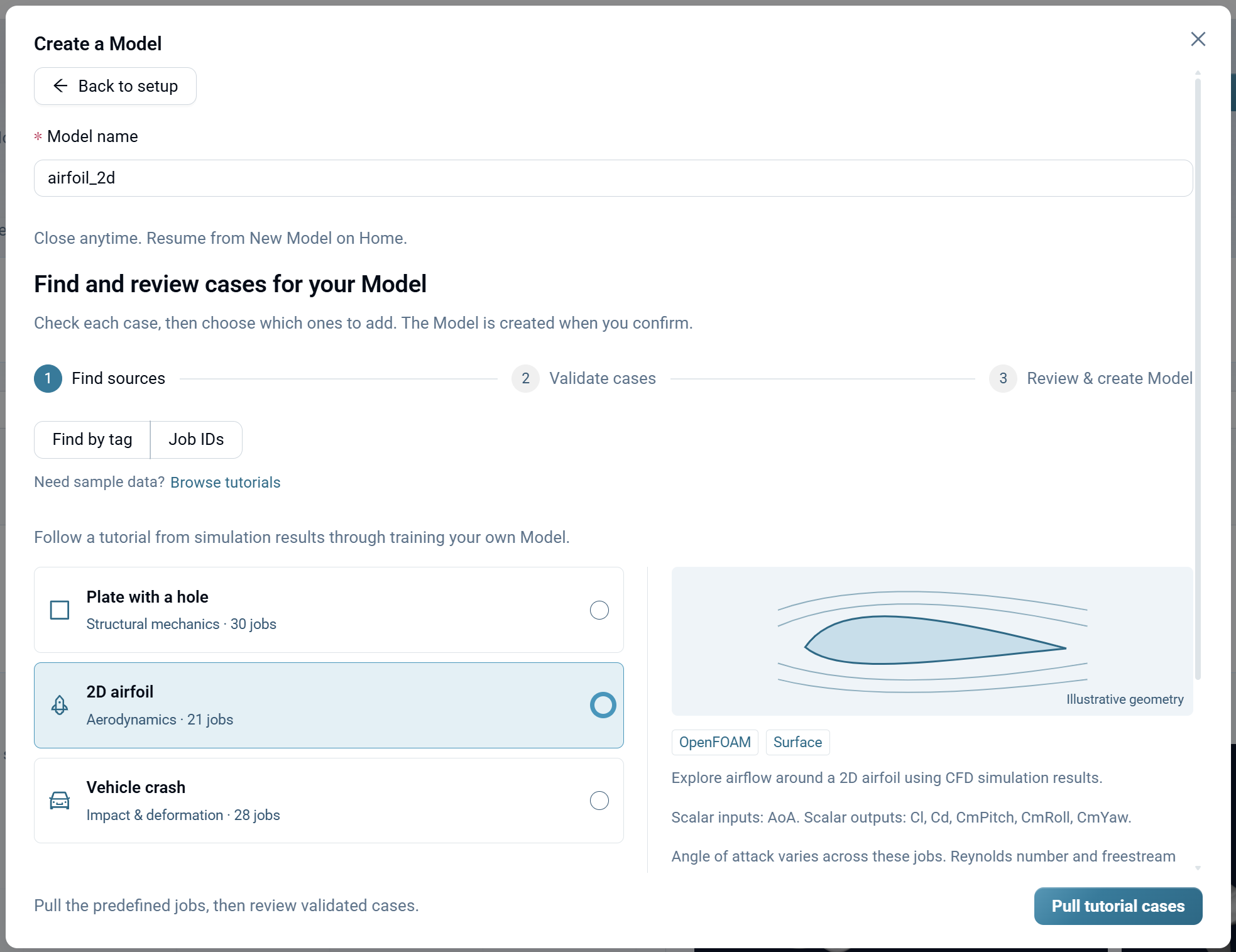
Find Your Simulation Data

Choose one of three methods to locate your simulation jobs:

Find by tag: Enter a job tag to pull all jobs with that tag. This is useful if you tagged your DOE runs consistently.

Job IDs: Enter specific Rescale job IDs separated by commas or line breaks. Use this when you have a known set of job IDs from a parameter sweep.

Browse tutorials: Select a pre-built tutorial example to follow the full workflow with sample data before running your own simulations.

Data agent: Select the AI-powered assistant that transforms historical simulation output into validated dataset cases. The agent reads output files from your completed Rescale jobs, identifies data structure and dependencies, checks license requirements, and prepares cases that match your model's field contract, with your approval at every step.

Validate Cases

Once you select a data source, AI Physics validates each case:

1. Checks data files: Verifies that each job has the required simulation output files produced by AI Extraction Automation.
2. Validates consistency: Ensures all cases have matching variable schemas (same solver, same output variables).
3. Flags issues: Identifies any invalid or incomplete cases that should be excluded.

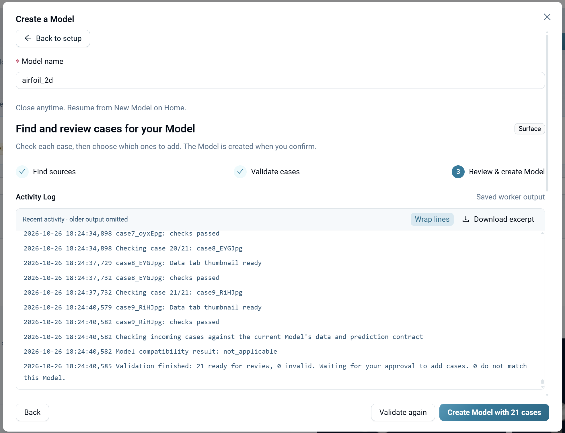
The Activity Log displays the validation progress and results. Review the summary:

• Cases ready for review: Valid cases that can be included in your model.
• Invalid cases: Cases with missing data or validation errors. These cannot be included.
• Cases that do not match this Model: Cases with incompatible data types or variable schemas.

Create the Model

Once validation completes successfully, click Create Model with [N] cases. The model is created and you're taken to the model's Data tab.

Configure Data

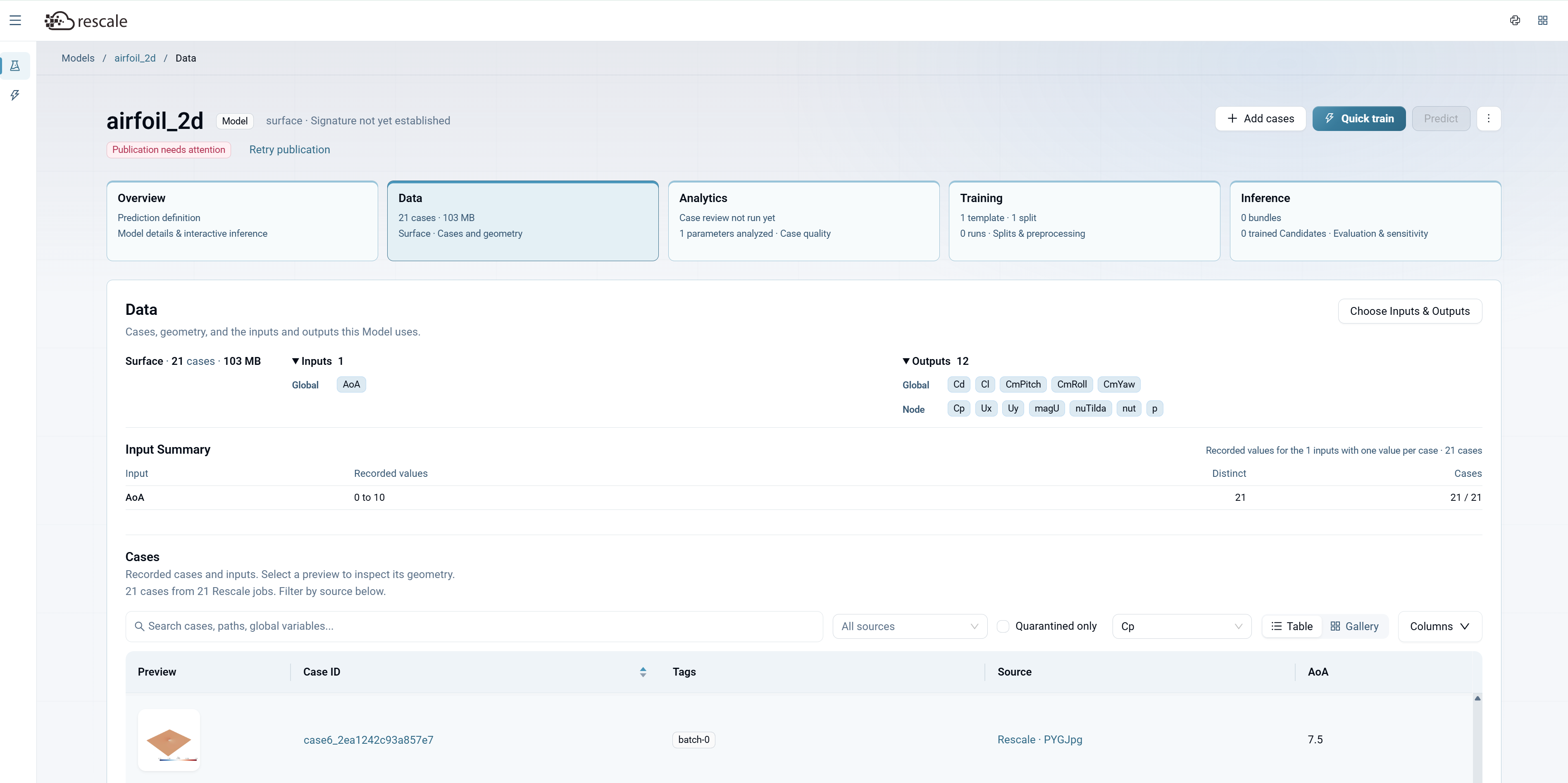
The Data tab shows all cases included in your model. Here you review the case list, inspect input and output variables, and configure which fields the model should use for training.

Review Cases

The Data tab displays:

• Case count and total data size: Summary of how many cases are included and the total size of the simulation data.
• Data type: Surface, Volume, or Scalar—set during model creation.
• Input and output summary: Lists the global input variables (from Custom Fields) and output variables (from simulation results).
• Cases table: Shows each case with preview thumbnail, Case ID, tags, source job, and input variable values.

Choose Inputs and Outputs

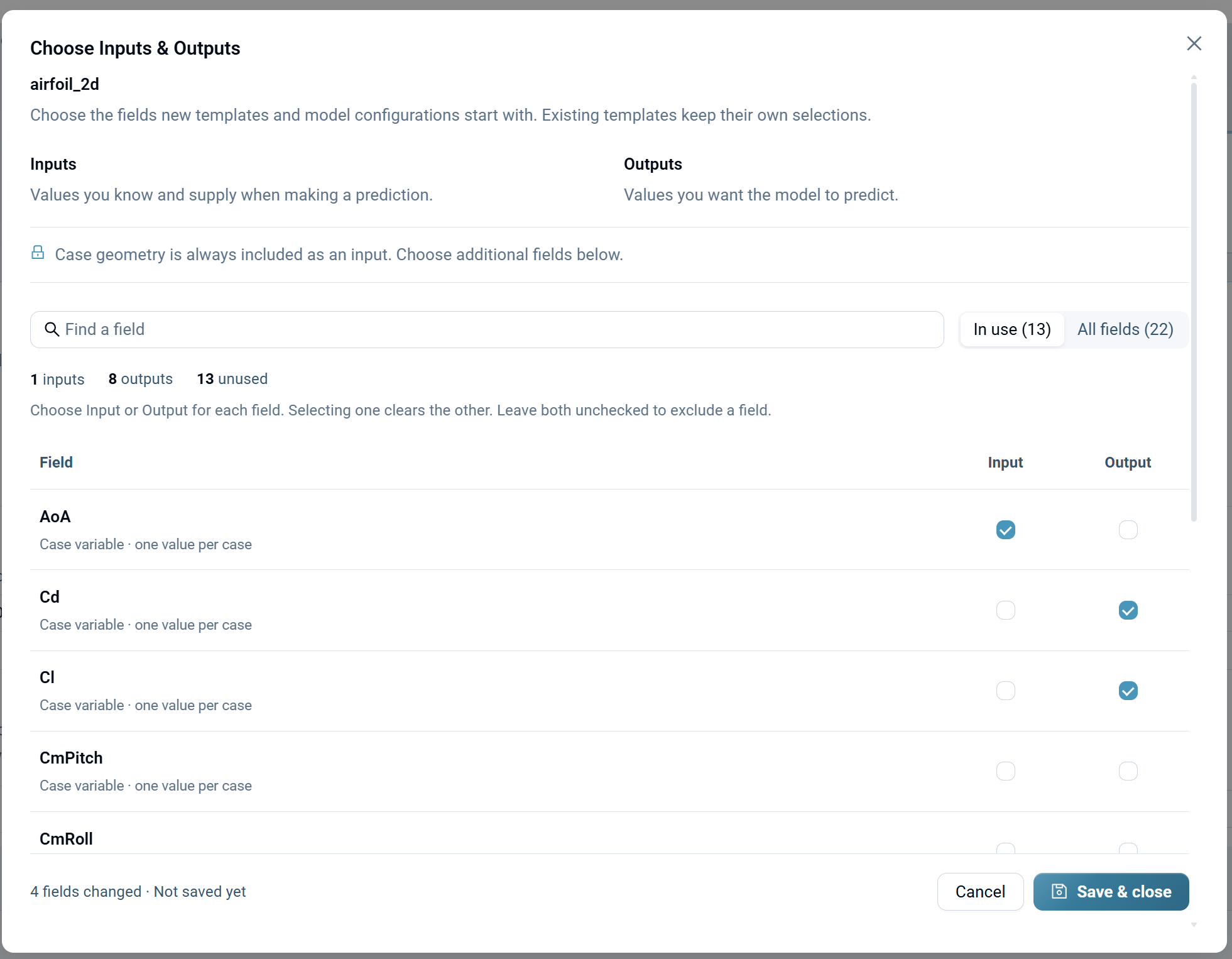
Click Choose Inputs & Outputs to configure which variables the model uses for training.

Inputs: Values you provide when making a prediction. These are typically design parameters or operating conditions extracted from Custom Fields (e.g., angle of attack, Mach number, Reynolds number). Case geometry is always included as an input.

Outputs: Values you want the model to predict. These come from your simulation results (e.g., pressure, velocity, temperature, drag coefficient, lift coefficient).

For each field in your data:

1. Check the Input box if the field is a known parameter you'll provide at inference time.
2. Check the Output box if the field is a value you want the model to predict.
3. Leave both unchecked to exclude the field from training.

Click Save & close when you're finished.

Review Analytics

The Analytics tab helps you assess data quality before training. It identifies outliers, evaluates your test/training split, and suggests ways to improve design space coverage.

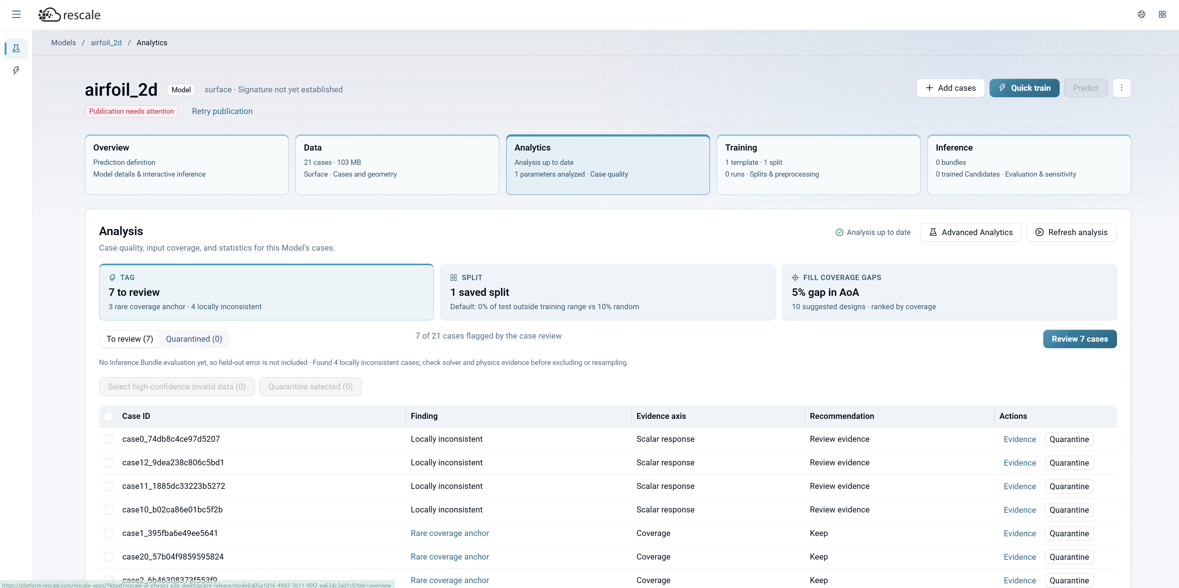
Navigate to the Analytics tab to see:

Case Review

Lists cases flagged for review based on statistical analysis:

• To review: Cases with potential outliers or unusual values. Check the evidence and decide whether to exclude the case or keep it.
• Quarantined: Cases you've marked for exclusion. They won't be used in training.

For each flagged case:

• Finding: Why the case was flagged (e.g., "Locally inconsistent", "Rare coverage anchor", "Scalar response").
• Evidence axis: Which variable triggered the flag.
• Recommendation: Whether to review evidence, keep, or exclude the case.
• Actions: Click Evidence to see detailed statistics, or Quarantine to exclude the case from training.

Saved Splits

Shows how your data is divided into training, validation, and test sets. A good split ensures both the training and test sets have similar coverage of your design space.

AI Physics recommends a split that:

• Reserves enough cases for validation and testing (typically 10-20% of total cases).
• Ensures all regions of your input space are represented in both training and test sets.

Coverage Gaps

Identifies regions of your design space with sparse data. If certain input combinations are underrepresented, the model may not generalize well to those regions.

For each gap, AI Physics provides:

• Description: Which region of the input space is under-covered.
• Suggestion: Recommended additional simulation runs to fill the gap.

Tip: Review the Analytics tab before launching training. Excluding outliers and ensuring good split coverage can significantly improve model accuracy.

Configure Training

Once your data is configured and reviewed, navigate to the Training tab to set up a training run.

Select a Training Template

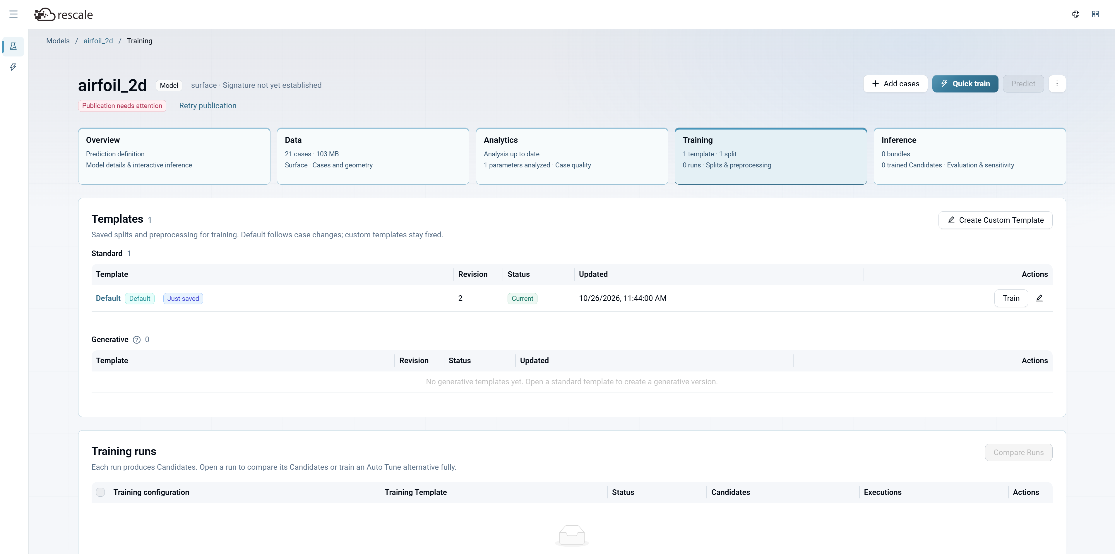
Templates capture your data configuration (selected inputs/outputs, case split, and normalization settings). When you first create a model, a Default template is automatically created with your current data settings.

Click Train next to the Default template to start a new training run.

Create a Training Run

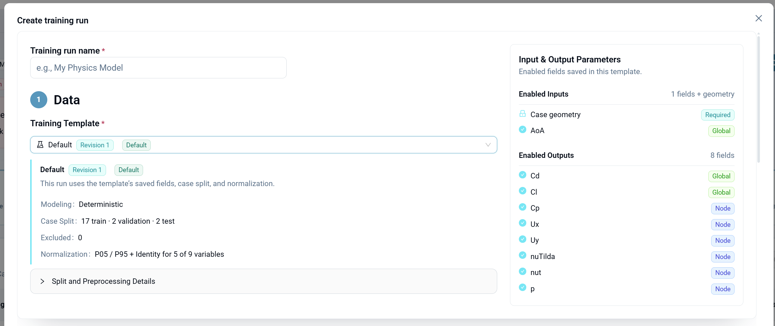
When you click Train, the Create training run dialog opens with three sections: Data, Configuration, and Hardware.

1. Data

Shows which model and training template you're using. The template defines:

• Modeling: Whether the model is deterministic (single prediction) or probabilistic (uncertainty ensemble).
• Case Split: How cases are divided into training, validation, and test sets (e.g., "17 train · 2 validation · 2 test").
• Excluded cases: How many cases have been quarantined.
• Normalization: Which normalization method is applied to inputs and outputs.

Expand Split and Preprocessing Details to see the full configuration.

You can click Change Template to select a different template if you've created multiple configurations.

2. Configuration

Choose how to configure training parameters.

Choose a Configuration Method

Select Auto Tune or Manual under Configuration Method.

Use Auto Tune when...	Use Manual when...
You want the best model without tuning expertise	You have specific hyperparameter constraints
You're training on a new dataset for the first time	You need full control over every training parameter
You want to explore multiple configurations efficiently	You're reproducing a prior experiment exactly

Auto Tune

Auto Tune automatically optimizes your surrogate model's hyperparameters and training configuration. You choose how long to search and Auto Tune handles the rest.

Select Your Model Architecture

Choose the architecture that matches your data type. Each tab displays a description and tags indicating supported use cases.

Architecture	Best for
TwoStreamTransformer	Highly efficient and suitable for both CFD and FEA use cases
DoMINO	Steady-state CFD surface variable prediction (e.g., surface pressure, wall shear stress, drag and lift coefficients)
Transolver / GeoTransolver	A geometry-aware transformer architecture designed for predictions over complex 3D geometries on unstructured meshes, where accurately capturing geometric relationships between mesh points is important
MeshGraphNet	A graph neural network architecture well-suited for FEA problems with complex deformation and stress field predictions

Set Search Duration

Auto Tune needs a time budget to explore configurations. Longer searches try more candidates and are more likely to find an optimal model.

Option	Duration	Best for
Quick Check	1 hour	Verifying your data pipeline works, getting a rough baseline
Baseline Search (Recommended)	6 hours	Most use cases — good balance of exploration and cost
Thorough Search	24 hours	Large or complex datasets where marginal accuracy gains matter
Custom	Set your own	When you know your compute budget or have specific time constraints

Note: Search time covers exploration and model selection only. Initial setup and final model polish happen afterward and do not count against this time.

Cost estimation: Your maximum Auto Tune cost is bounded by: search duration × hardware hourly rate.

Maximum time per epoch: If you want to specify a maximum runtime for each epoch you can use this setting. The default should be sufficient for most cases.

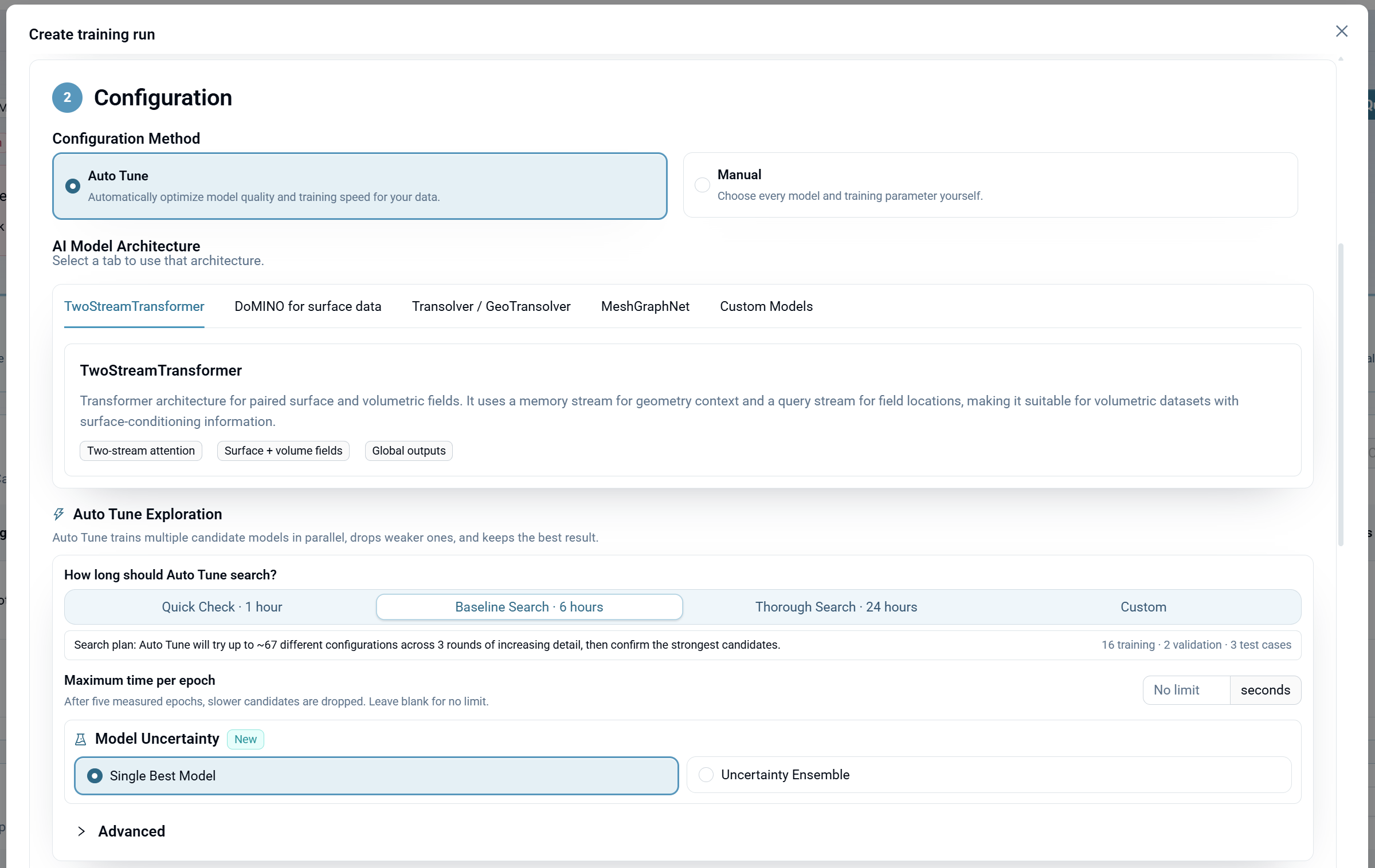
Advanced Settings (Optional)

Expand the Advanced: Population Initialization section to configure how Auto Tune initializes its search.

Candidate Initialization

Controls where Auto Tune gets its starting hyperparameters:

• Fresh population (default) — Every candidate starts from scratch with random hyperparameters. Use this for your first model on a dataset.
• Compatible prior runs — Seeds hyperparameters from compatible prior Auto Tune runs in your organization, while keeping model weights fresh. Use this when your team has trained similar models before and you want to benefit from that history. The current run's best hyperparameters are contributed back to the registry for future use.

Note: Compatible prior runs borrows the configuration recipe (learning rate, batch size, architecture settings) from prior experiments. It does not transfer trained model weights.

Optional Hyperparameter Seed

If you have a completed model of the same architecture trained on this dataset, you can use its hyperparameters as a starting point. This narrows the search space and can lead to faster convergence.

This option is only available when a compatible completed model exists. If you see "No compatible base models," no prior model of the selected architecture has been trained to completion on your current dataset.

3. Hardware

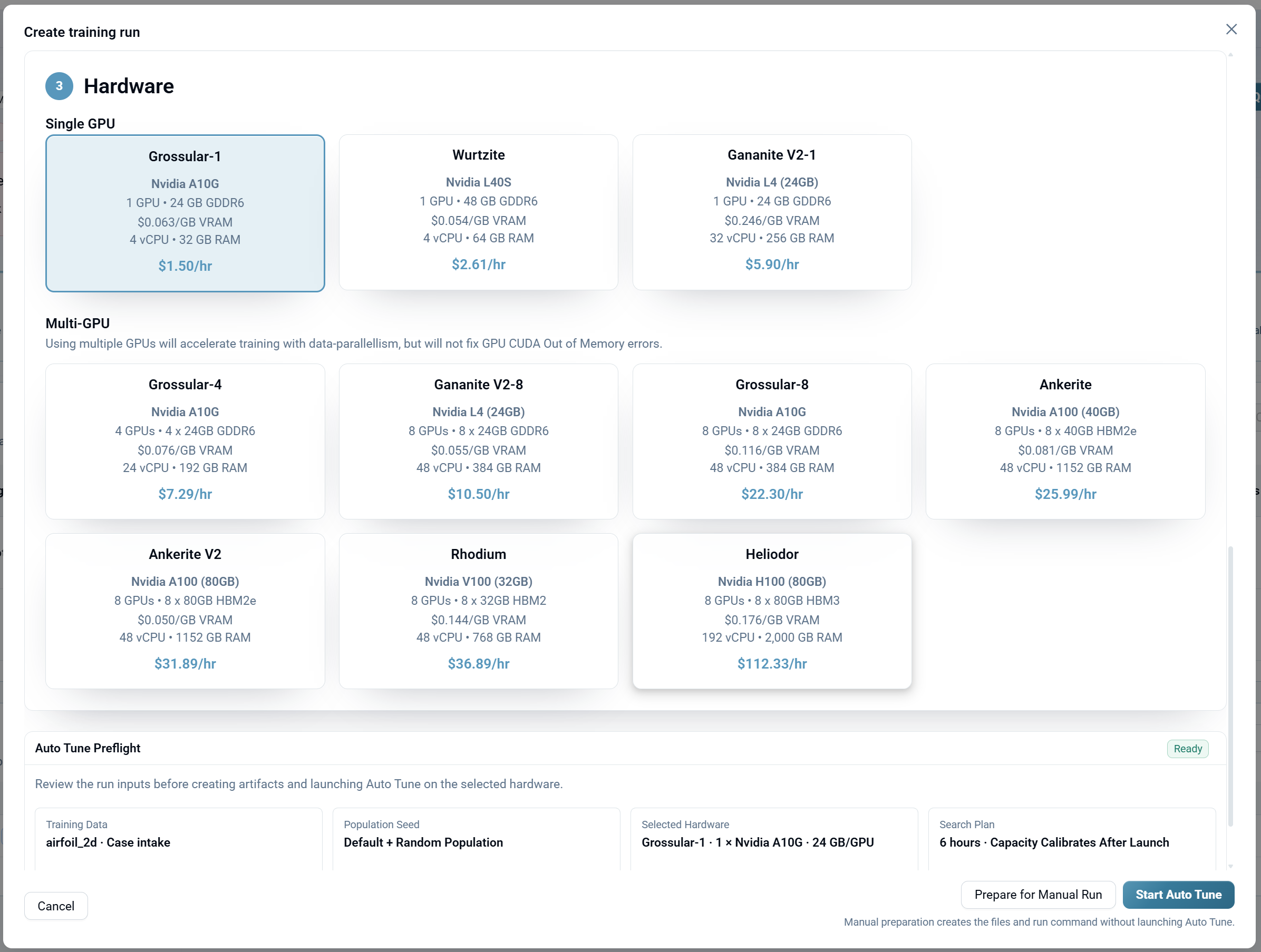
Choose a GPU configuration for training.

• Single GPU: Lower cost, suitable for smaller datasets and models. Options include Grossular-1 (Nvidia A10G), Wurtzite (Nvidia L40S), and Gananite V2-1 (Nvidia L4).
• Multi-GPU: Accelerates training with data-parallelism. Use when your model or batch size exceeds single-GPU memory. Options include Grossular-4/8, Gananite V2-8, Ankerite V2, and others. Note: Multi-GPU does not fix GPU CUDA Out of Memory errors; for those you need a card with more memory per GPU.

Each hardware option displays:

• GPU type and count
• VRAM per GPU
• vCPU and RAM
• Hourly cost

Launch Training

Once Data, Configuration and Hardware are set, the Auto Tune Preflight panel summarizes the run before anything is created. It shows four cards, Training Data, Population Seed, Selected Hardware and Search Plan, so you can confirm what you are about to spend compute on. When every required input is present the panel reports Ready, and starting the run creates the artifacts and launches the search on the workstation.

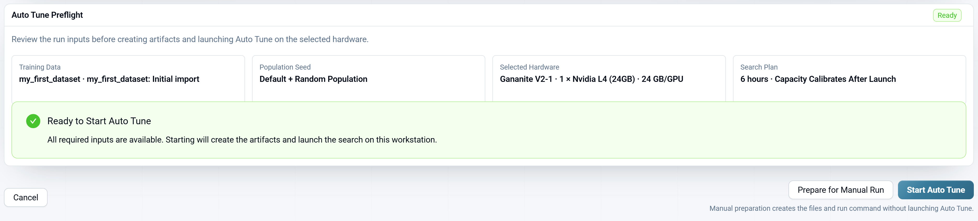
From the panel:

• For Auto Tune: Click Start Auto Tune to begin the hyperparameter search.
• For Manual: Click Prepare for Manual Run to generate training files, then click Start to begin training. Manual preparation writes the files and the run command without launching Auto Tune.

The training run begins and you're taken to the training progress view.

Monitor Training Progress

Training Curves

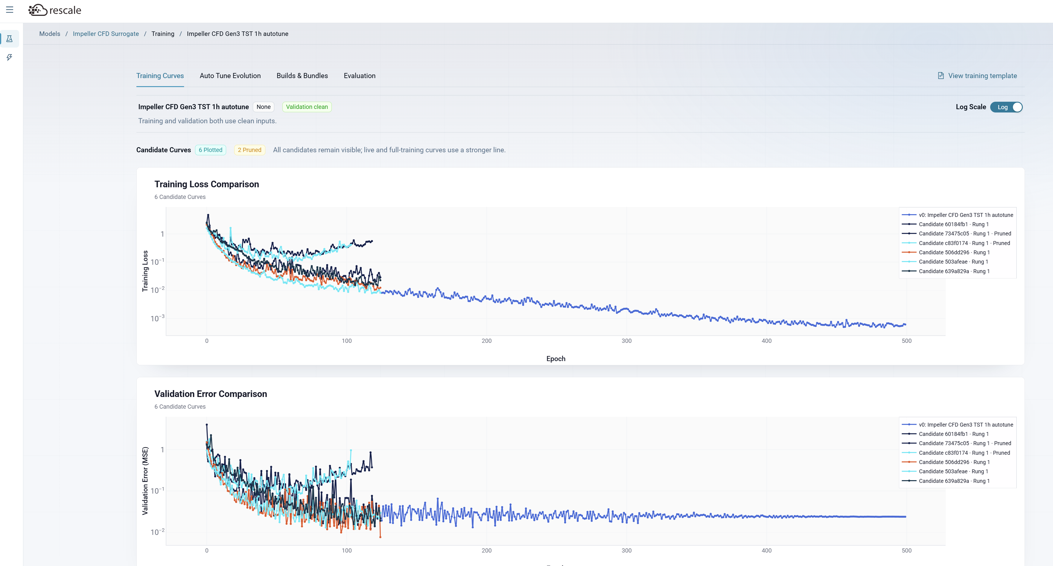
The Training Curves tab shows training and validation loss over time for all candidates in your training run.

Candidate Curves

Track multiple candidates simultaneously. The legend shows each candidate with its training status (e.g., "Rung 1", "Rung 2", "Paused"). All candidates remain visible for comparison, and a full training log is available for troubleshooting.

Training Loss Comparison

Plots training loss vs epoch for all candidates. Each candidate appears as a separate line. Lower training loss indicates the model is learning the training data patterns.

Validation Error Comparison

Plots validation error vs epoch for all candidates. Validation error on held-out data is the key metric for comparing candidates, since lower validation error means better generalization. Watch for candidates whose validation error plateaus or increases while training loss decreases (a sign of overfitting).

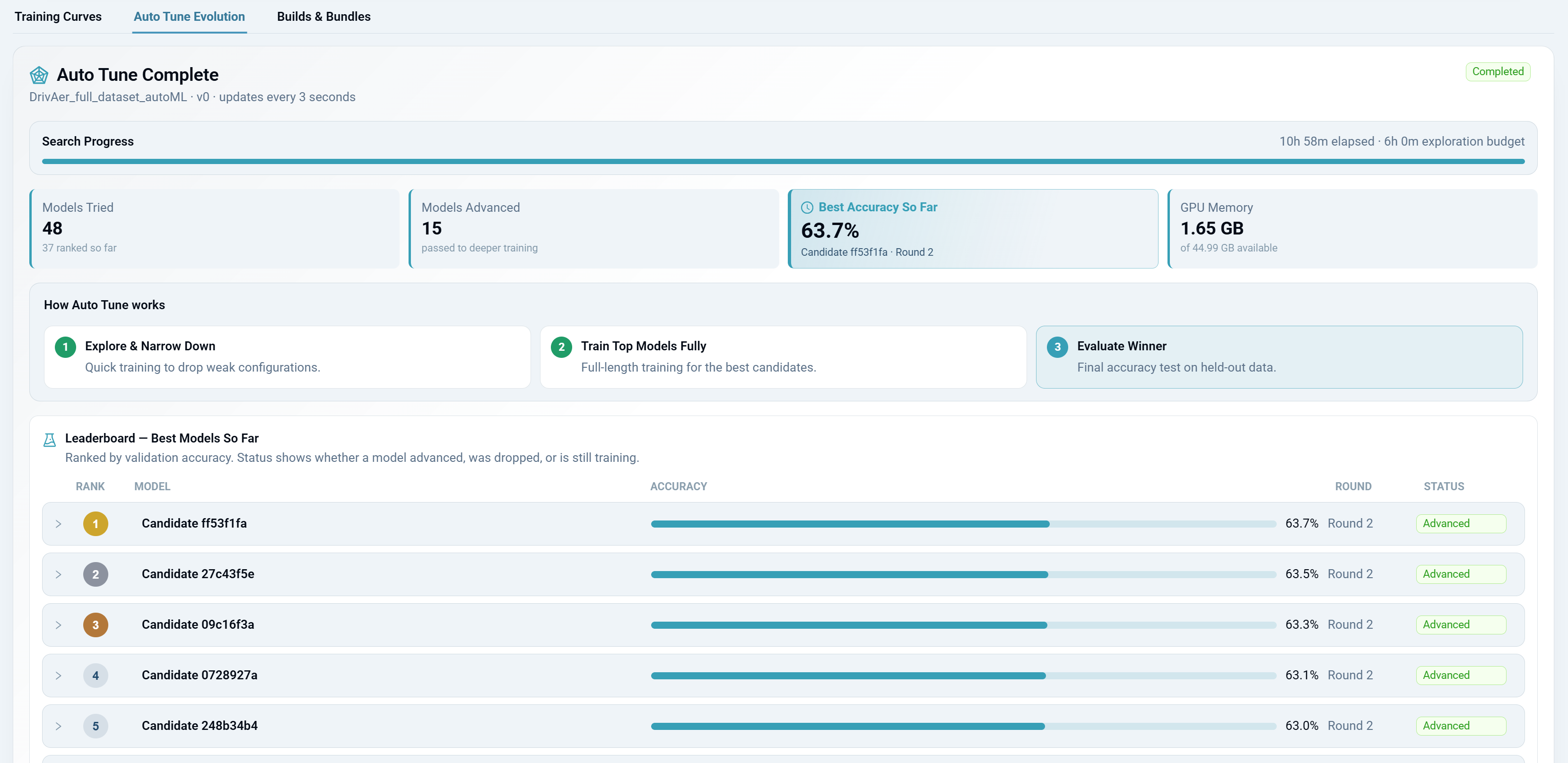
Auto Tune Evolution

Navigate to the Auto Tune Evolution tab to track hyperparameter search progress in real time.

Key Metrics

Metric	What it means
Models Tried	Candidates explored so far (out of planned total)
Models Advanced	Candidates promoted to full-length training
Best Accuracy So Far	Current best validation accuracy across all candidates
GPU Memory	Memory consumed (of total available on selected hardware)
Search Progress	Time elapsed and remaining in your search budget

How Auto Tune Works (3 Phases)

1. Explore & Narrow Down. Quick training runs evaluate many configurations. Weak candidates are dropped early to save compute.
2. Train Top Models Fully. Surviving candidates receive full-length training to reach their true potential.
3. Evaluate Winner. Final accuracy test on held-out data selects the best model.

Leaderboard

The Leaderboard — Best Models So Far ranks candidates by validation accuracy. Status shows whether a model advanced (promoted to deeper training), was dropped, or is still training.

Technical Details (Power Users)

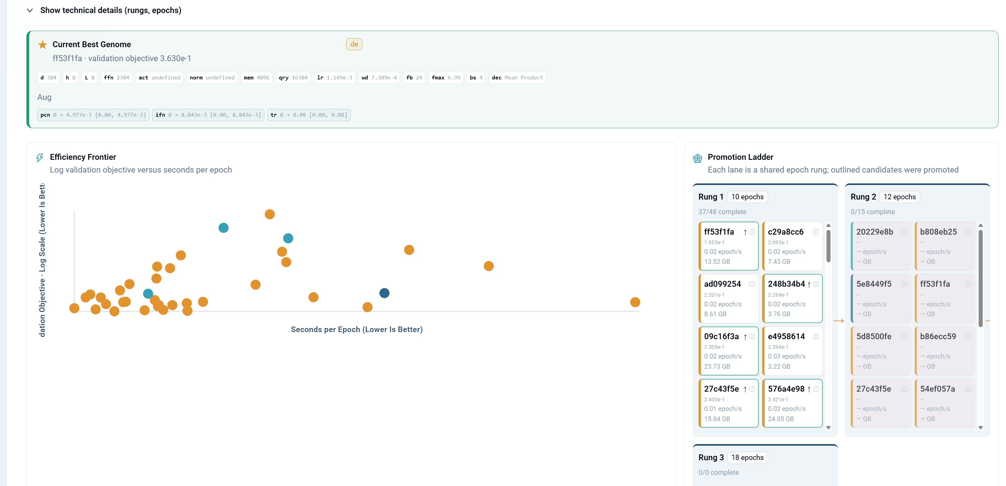
Expand Show technical details for deeper insight:

• Efficiency Frontier — Plots validation objective vs training cost (seconds per epoch). Identifies models that are both accurate and efficient.
• Promotion Ladder — Visualizes the rung system. Candidates must prove themselves at progressively longer epoch counts (e.g., Rung 1: 100 epochs → Rung 2: 200 epochs → Rung 3: 300 epochs) to advance.

Builds & Bundles

The Builds & Bundles tab shows training history and immutable model artifacts for creating inference bundles.

Training Runs

Lists all training runs for this model version (e.g., "Auto Tune · Completed"). Click a run to see its candidate portfolio and build artifacts.

Candidate Portfolio

Shows all candidates evaluated during the training run, ranked by validation performance:

• Rank: Candidate ranking by validation score
• Candidate: Candidate ID (e.g., 583afea6, 639ab29a)
• Validation: Validation score (lower is better for error metrics)
• Fidelity: Training checkpoint (e.g., 125 epochs)
• Checkpoint: Status (Retained or discarded)
• Actions: Train Fully button to extend a retained candidate to full training

Only completed Model Builds are eligible for standard inference bundles. Retained candidates are partial-fidelity checkpoints that can be trained to completion.

Model Builds

Lists finalized model builds ready for inference:

• Build: Build ID (e.g., e98eb65)
• Architecture: Model architecture used (e.g., TwoStreamTransformer)
• Source: Which candidate the build came from (e.g., Candidate 9cbd0b67)
• Actions: Build Bundle button to package the model for inference

Inference Bundles

Lists inference bundles created from Model Builds. Each bundle packages a model for deployment in AI Physics Inference, local inference, or CAD tools.

Evaluation

The Evaluation tab provides comprehensive model quality assessment after training completes.

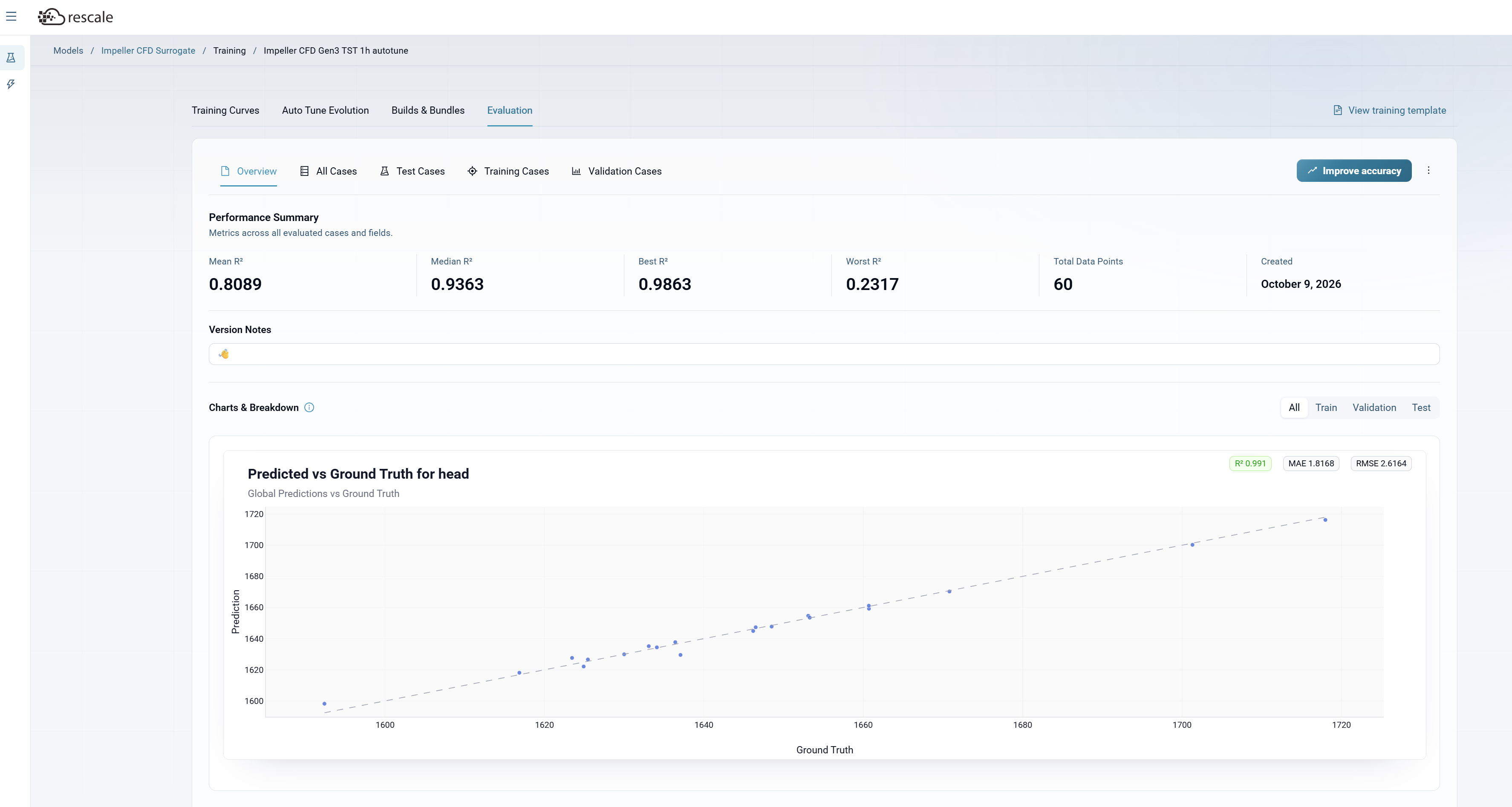
Performance Summary

Metrics across all evaluated cases and fields:

• Mean R²: Average R² across all output fields
• Median R²: Median R² across all output fields (less sensitive to outliers than mean)
• Best R²: Highest R² achieved on any single field
• Worst R²: Lowest R² achieved on any single field
• Total Data Points: Number of cases evaluated
• Created: When the model version was created

Case Views

Navigate between case subsets using the tabs:

• Overview: Summary statistics and aggregate visualizations across all cases
• All Cases: Predictions and errors across training, validation, and test sets combined
• Test Cases: Performance on held-out test data (the definitive quality metric)
• Training Cases: Performance on training data
• Validation Cases: Performance on validation data used during hyperparameter tuning

Charts & Breakdown

Filter charts by All, Train, Validation, or Test to focus on specific case subsets.

Predicted vs Ground Truth: Scatter plots comparing model predictions to true simulation values for each output field. Points near the diagonal line indicate accurate predictions. Each chart displays:

• R²: Coefficient of determination (1.0 = perfect predictions)
• MAE: Mean Absolute Error
• RMSE: Root Mean Squared Error

Version Notes: Optional notes field for recording observations about this model version (e.g., "Best performance on high-RPM cases", "Trained with expanded dataset").

Click Improve accuracy to launch a new training run with adjusted hyperparameters or additional data.

Understanding Accuracy vs R²

You'll see two different metrics during and after training. They measure different things:

Metric	Where you see it	What it measures
Accuracy (%)	Auto Tune leaderboard during search	Internal search metric used to rank and promote candidates. Measures how well a candidate performs relative to others during exploration.
R² (Performance)	Evaluation tab after completion	Final evaluation on held-out test data. The definitive quality metric for your model. Measures how well predictions match true values on data the model never trained on.

These metrics can tell different stories. A candidate with high leaderboard accuracy during search may produce a lower R² on final evaluation because held-out test data presents harder cases than the training split. Always use R² as your ground truth for model quality.

Interpreting R²

R² value	Interpretation	Action
Close to 1.0	Strong model — predictions closely match true values	Deploy for inference
Close to 0	Model is no better than predicting the average	Increase search duration or add more training data
Negative	Model performs worse than predicting the average	Try a longer search, more data, or a different architecture

Important: Auto Tune completing successfully does not guarantee a high-quality model. Always check the R² score in the Evaluation tab before deploying.

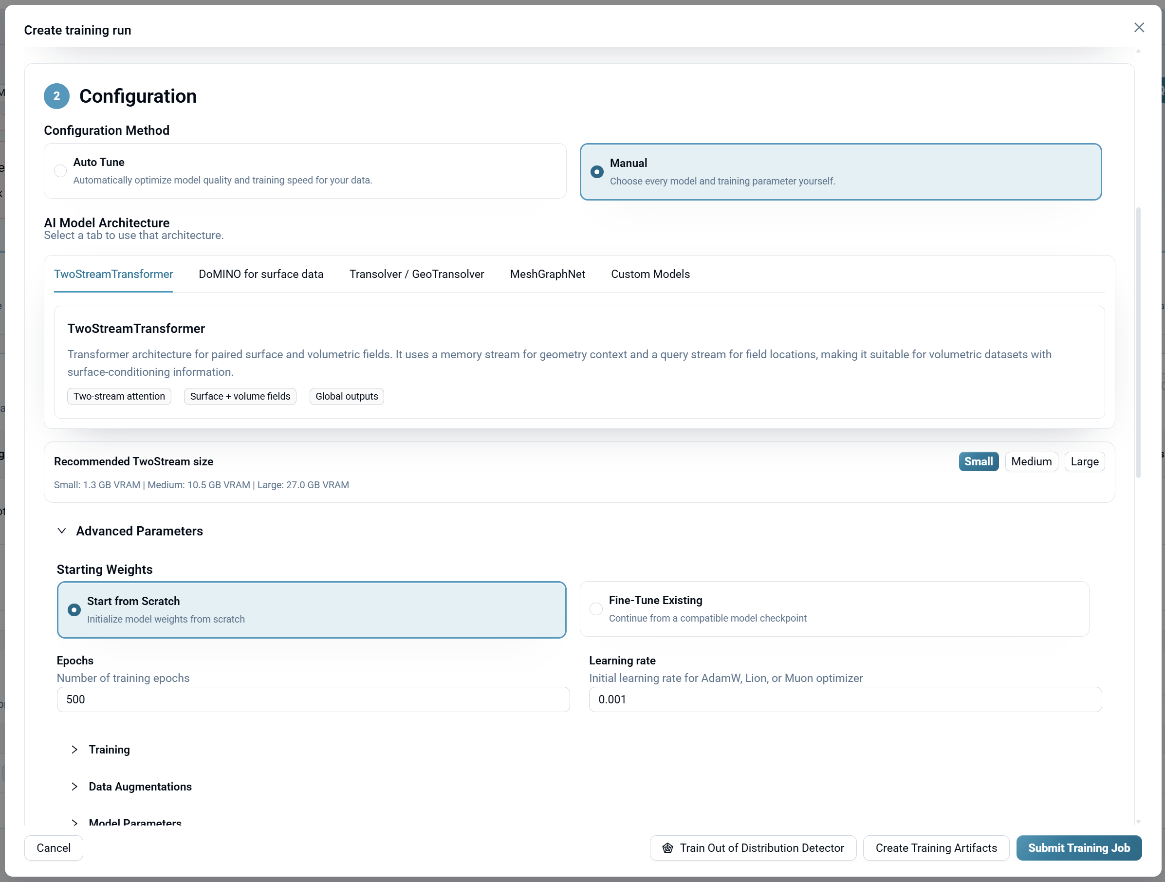
Manual Configuration

Select Manual when you need full control over every training parameter.

In Manual mode, you configure:

1. Model architecture: same four options as Auto Tune (TwoStreamTransformer, DoMINO, Transolver/GeoTransolver, MeshGraphNet)
2. Hyperparameters: learning rate, batch size, number of epochs, optimizer settings, and architecture-specific parameters
3. Hardware: same GPU selection as Auto Tune

Default parameters are suitable for most use cases. Adjust individual parameters only if you have specific requirements or are iterating on a prior experiment.

Fine-Tuning an Existing Model

To improve a previously trained model:

1. Select the existing model from the Select Model dropdown when creating a new model.
2. The new version inherits the prior model's architecture and configuration as a starting point.
3. With Auto Tune, use the Optional Hyperparameter Seed in Advanced settings to seed from the prior model's hyperparameters.
4. With Manual, adjust specific parameters and retrain.

This is useful when you've added new simulation data to your dataset or want to improve accuracy on specific regions of the design space.

Troubleshooting

Auto Tune Failed

If you see "Auto Tune did not complete any valid trials," the search budget was likely too short for your data complexity:

• "Measured epoch cost leaves room for fewer than three additional search trials" — Your data/architecture combination is expensive per epoch. Increase your search budget (try Baseline Search or Thorough Search) to allow broader exploration.
• Verify that your training dataset is correctly formatted and accessible.
• Try a different architecture if the failure persists.

Low R² After Completion

If your model completes but shows a low or negative R²:

1. Increase search duration. A Quick Check may not explore enough candidates for complex datasets.
2. Add more training data. More simulation samples improve generalization.
3. Try a different architecture. Some architectures perform better on certain data types.
4. Check data quality. Ensure your simulation outputs don't contain errors or extreme outliers.

GPU Out of Memory

If training fails due to GPU memory:

• Select hardware with more VRAM (check the GPU Memory metric during training).
• Note that switching to Multi-GPU does not fix CUDA Out of Memory errors — you need a card with more memory per GPU.

What's Next

After your model completes with acceptable R²:

• Deploy for inference — Click the inference icon in the Versions table to use the model for predictions on new data. See Running Inference.
• Compare versions — Train multiple versions with different settings and compare their R² scores and training curves.
• Iterate — Use the winning model's hyperparameters as a seed for future Auto Tune runs via the Cross-Dataset Registry or Optional Hyperparameter Seed.

FAQ

Do I need to create an AI Dataset separately before creating a model? No. In the current AI Physics workflow, model creation and data selection happen together. When you create a new model, you select your simulation jobs, validate cases, and configure inputs and outputs, all in one flow.

What happens if I need to add more simulation data later? You can add cases to an existing model by clicking Add cases in the Data tab. This is useful when you've run additional simulations and want to retrain with more data.

Do I need machine learning experience to use Auto Tune? No. Auto Tune is designed for simulation engineers, not ML experts. You choose a search duration and AI Physics handles hyperparameter tuning automatically.

How long does Auto Tune actually take? The search duration you select (1, 6, or 24 hours) covers candidate exploration only. Initial setup and final model polish add extra time.

Can I stop Auto Tune early if I see a good candidate? Currently, Auto Tune must complete its full search to produce a usable model. Early stopping with partial results is not supported.

How do I know if my model is overfitting? Review the Training Curves tab. If training loss continues to decrease while validation loss plateaus or increases, your model is overfitting. Solutions: increase dropout, reduce model complexity, or add more training data.

Should I review Analytics before every training run? Yes, it's recommended. The Analytics tab helps you catch outliers and identify coverage gaps before you invest compute time in training. Excluding bad cases and ensuring good split coverage can save hours of retraining.

When should I use the Dataset Creation Agent vs. adding cases by Job IDs? Use Job IDs/tags (the default method) when your jobs already have AI Extraction and Metadata Extraction Automations enabled, which is the simplest path. Use the Dataset Creation Agent when:

• Your simulation files need solver-specific conversion (the agent handles license detection and conversion)
• You want guided assistance mapping complex simulation outputs to your model's field contract
• You're working with historical jobs that may not have had Automations enabled

Does the Dataset Creation Agent check out a solver license? Not during inspection. The agent assesses whether a license is needed and records the configuration. A license is only used if files require solver-based conversion during the Prepare step. If direct-read extraction is possible, no license is checked out.

What happens if a case fails validation in the Dataset Creation Agent? Failed cases remain in the scratch area and aren't added to the dataset. You can inspect them in the notebook, correct the issue, and click Validate again. Common failures include missing required fields or mismatched field names.

Can I merge, split or decimate a dataset after it exists? Yes. Those operations run from the Data tab in AI Physics Training. See Working with AI datasets, which also covers the Notebook Copilot and mesh decimation.